2. Content
2.1 Question 1
2.1.1 Read Data
I use 3 years data for the question as experiment, 1st year data is burn-in data for statistical modelling and prediction purpose while following 2 years data for forecasting and staking. There have 252 trading days within a year.
## get currency dataset online.
## http://stackoverflow.com/questions/24219694/get-symbols-quantmod-ohlc-currency-data
#'@ getFX('USD/JPY', from = '2014-01-01', to = '2017-01-20')

## getFX() doesn't shows Op, Hi, Lo, Cl price but only price. Therefore no idea to place bets.
#'@ USDJPY <- getSymbols('JPY=X', src = 'yahoo', from = '2014-01-01',
#'@                      to = '2017-01-20', auto.assign = FALSE)
#'@ names(USDJPY) <- str_replace_all(names(USDJPY), 'JPY=X', 'USDJPY')
#'@ USDJPY <- xts(USDJPY[, -1], order.by = USDJPY$Date)

#'@ saveRDS(USDJPY, './data/USDJPY.rds')
USDJPY <- read_rds(path = './data/USDJPY.rds')
mbase <- USDJPY

## dateID
dateID <- index(mbase)
dateID0 <- ymd('2015-01-01')
dateID <- dateID[dateID > dateID0]dim(mbase)## [1] 797 6summary(mbase) %>% kable(width = 'auto')| Index | USDJPY.Open | USDJPY.High | USDJPY.Low | USDJPY.Close | USDJPY.Volume | USDJPY.Adjusted | |
|---|---|---|---|---|---|---|---|
| Min. :2014-01-01 | Min. : 99.89 | Min. :100.4 | Min. : 99.57 | Min. : 99.91 | Min. :0 | Min. : 99.91 | |
| 1st Qu.:2014-10-07 | 1st Qu.:103.18 | 1st Qu.:103.6 | 1st Qu.:102.79 | 1st Qu.:103.19 | 1st Qu.:0 | 1st Qu.:103.19 | |
| Median :2015-07-13 | Median :112.50 | Median :113.0 | Median :112.03 | Median :112.49 | Median :0 | Median :112.49 | |
| Mean :2015-07-12 | Mean :111.95 | Mean :112.3 | Mean :111.53 | Mean :111.95 | Mean :0 | Mean :111.95 | |
| 3rd Qu.:2016-04-18 | 3rd Qu.:119.76 | 3rd Qu.:120.1 | 3rd Qu.:119.25 | 3rd Qu.:119.78 | 3rd Qu.:0 | 3rd Qu.:119.78 | |
| Max. :2017-01-20 | Max. :125.60 | Max. :125.8 | Max. :124.97 | Max. :125.63 | Max. :0 | Max. :125.63 |
2.1.2 Statistical Modelling
2.1.2.1 ARIMA vs ETS
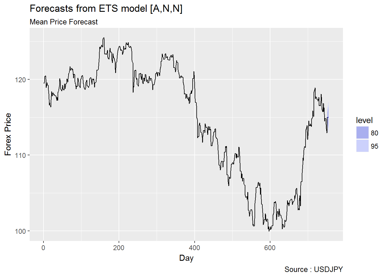
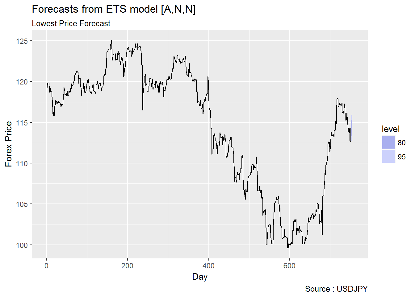
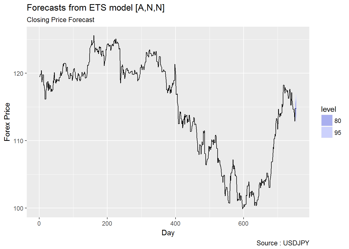
Remarks : Here I try to predict the sell/buy price and also settled price. However just noticed the question asking about prediction of the variance2 The profit is made based on the range of variance Hi-Lo price but not the accuracy of the highest, lowest or closing price. based on mean price. I can also use the focasted highest and forecasted lowest price for variance prediction as well. However I will conduct another study and answer for the variance with Garch models.
Below are some articles with regards exponential smoothing.
- Recent Advances in Robust Statistics: Theory and Applications
- Error, trend, seasonality - ets and its forecast model friends
- A study of outliers in the exponential smoothing approach to forecasting
- 8.10 ARIMA vs ETS
- Introduction to ARIMA : nonseasonal models
It is a common myth that ARIMA models are more general than exponential smoothing. While linear exponential smoothing models are all special cases of ARIMA models, the non-linear exponential smoothing models have no equivalent ARIMA counterparts. There are also many ARIMA models that have no exponential smoothing counterparts. In particular, every ETS model3 forecast::ets() : Usually a three-character string identifying method using the framework terminology of Hyndman et al. (2002) and Hyndman et al. (2008). The first letter denotes the error type (“A”, “M” or “Z”); the second letter denotes the trend type (“N”,“A”,“M” or “Z”); and the third letter denotes the season type (“N”,“A”,“M” or “Z”). In all cases, “N”=none, “A”=additive, “M”=multiplicative and “Z”=automatically selected. So, for example, “ANN” is simple exponential smoothing with additive errors, “MAM” is multiplicative Holt-Winters’ method with multiplicative errors, and so on. It is also possible for the model to be of class “ets”, and equal to the output from a previous call to ets. In this case, the same model is fitted to y without re-estimating any smoothing parameters. See also the use.initial.values argument. is non-stationary, while ARIMA models can be stationary.
The ETS models with seasonality or non-damped trend or both have two unit roots (i.e., they need two levels of differencing to make them stationary). All other ETS models have one unit root (they need one level of differencing to make them stationary).
The following table gives some equivalence relationships for the two classes of models.
| ETS model | ARIMA model | Parameters |
|---|---|---|
| \(ETS(A, N, N)\) | \(ARIMA(0, 1, 1)\) | \(θ_{1} = α − 1\) |
| \(ETS(A, A, N)\) | \(ARIMA(0, 2, 2)\) | \(θ_{1} = α + β − 2\) |
| \(θ_{2} = 1 − α\) | ||
| \(ETS(A, A_{d}, N)\) | \(ARIMA(1, 1, 2)\) | \(ϕ_{1} = ϕ\) |
| \(θ_{1} = α + ϕβ − 1 − ϕ\) | ||
| \(θ_{2} = (1 − α)ϕ\) | ||
| \(ETS(A, N, A)\) | \(ARIMA(0, 0, m)(0, 1, 0)_{m}\) | |
| \(ETS(A, A, A)\) | \(ARIMA(0, 1, m+1)(0, 1, 0)_{m}\) | |
| \(ETS(A, A_{d}, A)\) | \(ARIMA(1, 0, m+1)(0, 1, 0)_{m}\) |
For the seasonal models, there are a large number of restrictions on the ARIMA parameters.
Kindly refer to 8.10 ARIMA vs ETS for further details.
## Modelling Auto Arima focasting data.
#'@ fitAutoArima.op <- suppressAll(simAutoArima(USDJPY, .prCat = 'Op')) #will take a minute
#'@ saveRDS(fitAutoArima.op, './data/fitAutoArima.op.rds')

#'@ fitAutoArima.hi <- suppressAll(simAutoArima(USDJPY, .prCat = 'Hi')) #will take a minute
#'@ saveRDS(fitAutoArima.hi, './data/fitAutoArima.hi.rds')

#'@ fitAutoArima.mn <- suppressAll(simAutoArima(USDJPY, .prCat = 'Mn')) #will take a minute
#'@ saveRDS(fitAutoArima.mn, './data/fitAutoArima.mn.rds')

#'@ fitAutoArima.lo <- suppressAll(simAutoArima(USDJPY, .prCat = 'Lo')) #will take a minute
#'@ saveRDS(fitAutoArima.lo, './data/fitAutoArima.lo.rds')

#'@ fitAutoArima.cl <- suppressAll(simAutoArima(USDJPY, .prCat = 'Cl')) #will take a minute
#'@ saveRDS(fitAutoArima.cl, './data/fitAutoArima.cl.rds')

fitAutoArima.op <- readRDS('./data/fitAutoArima.op.rds')
fitAutoArima.hi <- readRDS('./data/fitAutoArima.hi.rds')
fitAutoArima.mn <- readRDS('./data/fitAutoArima.mn.rds')
fitAutoArima.lo <- readRDS('./data/fitAutoArima.lo.rds')
fitAutoArima.cl <- readRDS('./data/fitAutoArima.cl.rds')
## Modelling ETS focasting data.
#'@ fitETS.op <- suppressAll(simETS(USDJPY, .prCat = 'Op')) #will take a minute
#'@ saveRDS(fitETS.op, './data/fitETS.op.rds')
#'@ fitETS.hi <- suppressAll(simETS(USDJPY, .prCat = 'Hi')) #will take a minute
#'@ saveRDS(fitETS.hi, './data/fitETS.hi.rds')
#'@ fitETS.mn <- suppressAll(simETS(USDJPY, .prCat = 'Mn')) #will take a minute
#'@ saveRDS(fitETS.mn, './data/fitETS.mn.rds')
#'@ fitETS.lo <- suppressAll(simETS(USDJPY, .prCat = 'Lo')) #will take a minute
#'@ saveRDS(fitETS.lo, './data/fitETS.lo.rds')
#'@ fitETS.cl <- suppressAll(simETS(USDJPY, .prCat = 'Cl')) #will take a minute
#'@ saveRDS(fitETS.cl, './data/fitETS.cl.rds')
fitETS.op <- readRDS('./data/fitETS.op.rds')
fitETS.hi <- readRDS('./data/fitETS.hi.rds')
fitETS.mn <- readRDS('./data/fitETS.mn.rds')
fitETS.lo <- readRDS('./data/fitETS.lo.rds')
fitETS.cl <- readRDS('./data/fitETS.cl.rds')Application of MCMC
Need to refer to MCMC since I am using exponential smoothing models…
## Here I test the accuracy of forecasting of ets ZZZ model 1.

## Test the models
## opened price fit data
summary(lm(Point.Forecast~ USDJPY.Close, data = fitETS.op))
##
## Call:
## lm(formula = Point.Forecast ~ USDJPY.Close, data = fitETS.op)
##
## Residuals:
## Min 1Q Median 3Q Max
## -2.4353 -0.4004 -0.0269 0.3998 3.3978
##
## Coefficients:
## Estimate Std. Error t value Pr(>|t|)
## (Intercept) 0.180332 0.490019 0.368 0.713
## USDJPY.Close 0.998722 0.004256 234.666 <2e-16 ***
## ---
## Signif. codes: 0 '***' 0.001 '**' 0.01 '*' 0.05 '.' 0.1 ' ' 1
##
## Residual standard error: 0.7286 on 533 degrees of freedom
## (216 observations deleted due to missingness)
## Multiple R-squared: 0.9904, Adjusted R-squared: 0.9904
## F-statistic: 5.507e+04 on 1 and 533 DF, p-value: < 2.2e-16summary(MCMCregress(Point.Forecast~ USDJPY.Close, data = fitETS.op))##
## Iterations = 1001:11000
## Thinning interval = 1
## Number of chains = 1
## Sample size per chain = 10000
##
## 1. Empirical mean and standard deviation for each variable,
## plus standard error of the mean:
##
## Mean SD Naive SE Time-series SE
## (Intercept) 0.1808 0.489606 4.896e-03 4.896e-03
## USDJPY.Close 0.9987 0.004257 4.257e-05 4.257e-05
## sigma2 0.5330 0.033014 3.301e-04 3.301e-04
##
## 2. Quantiles for each variable:
##
## 2.5% 25% 50% 75% 97.5%
## (Intercept) -0.7795 -0.1487 0.1848 0.5094 1.1441
## USDJPY.Close 0.9904 0.9959 0.9987 1.0016 1.0070
## sigma2 0.4716 0.5100 0.5317 0.5549 0.6009## highest price fit data
summary(lm(Point.Forecast~ USDJPY.Close, data = fitETS.hi))##
## Call:
## lm(formula = Point.Forecast ~ USDJPY.Close, data = fitETS.hi)
##
## Residuals:
## Min 1Q Median 3Q Max
## -2.3422 -0.3298 -0.0987 0.2166 3.2868
##
## Coefficients:
## Estimate Std. Error t value Pr(>|t|)
## (Intercept) 1.140616 0.379253 3.008 0.00276 **
## USDJPY.Close 0.993982 0.003294 301.765 < 2e-16 ***
## ---
## Signif. codes: 0 '***' 0.001 '**' 0.01 '*' 0.05 '.' 0.1 ' ' 1
##
## Residual standard error: 0.5639 on 533 degrees of freedom
## (216 observations deleted due to missingness)
## Multiple R-squared: 0.9942, Adjusted R-squared: 0.9942
## F-statistic: 9.106e+04 on 1 and 533 DF, p-value: < 2.2e-16summary(MCMCregress(Point.Forecast~ USDJPY.Close, data = fitETS.hi))##
## Iterations = 1001:11000
## Thinning interval = 1
## Number of chains = 1
## Sample size per chain = 10000
##
## 1. Empirical mean and standard deviation for each variable,
## plus standard error of the mean:
##
## Mean SD Naive SE Time-series SE
## (Intercept) 1.1410 0.378933 3.789e-03 3.789e-03
## USDJPY.Close 0.9940 0.003295 3.295e-05 3.295e-05
## sigma2 0.3193 0.019776 1.978e-04 1.978e-04
##
## 2. Quantiles for each variable:
##
## 2.5% 25% 50% 75% 97.5%
## (Intercept) 0.3978 0.8860 1.1441 1.3953 1.8865
## USDJPY.Close 0.9875 0.9918 0.9939 0.9962 1.0004
## sigma2 0.2825 0.3055 0.3185 0.3324 0.3599## mean price fit data (mean price of daily highest and lowest price)
summary(lm(Point.Forecast~ USDJPY.Close, data = fitETS.mn))##
## Call:
## lm(formula = Point.Forecast ~ USDJPY.Close, data = fitETS.mn)
##
## Residuals:
## Min 1Q Median 3Q Max
## -2.55047 -0.26416 -0.00996 0.26743 1.81654
##
## Coefficients:
## Estimate Std. Error t value Pr(>|t|)
## (Intercept) 0.106616 0.326718 0.326 0.744
## USDJPY.Close 0.999098 0.002838 352.091 <2e-16 ***
## ---
## Signif. codes: 0 '***' 0.001 '**' 0.01 '*' 0.05 '.' 0.1 ' ' 1
##
## Residual standard error: 0.4858 on 533 degrees of freedom
## (216 observations deleted due to missingness)
## Multiple R-squared: 0.9957, Adjusted R-squared: 0.9957
## F-statistic: 1.24e+05 on 1 and 533 DF, p-value: < 2.2e-16summary(MCMCregress(Point.Forecast~ USDJPY.Close, data = fitETS.mn))##
## Iterations = 1001:11000
## Thinning interval = 1
## Number of chains = 1
## Sample size per chain = 10000
##
## 1. Empirical mean and standard deviation for each variable,
## plus standard error of the mean:
##
## Mean SD Naive SE Time-series SE
## (Intercept) 0.1069 0.326443 3.264e-03 3.264e-03
## USDJPY.Close 0.9991 0.002838 2.838e-05 2.838e-05
## sigma2 0.2369 0.014676 1.468e-04 1.468e-04
##
## 2. Quantiles for each variable:
##
## 2.5% 25% 50% 75% 97.5%
## (Intercept) -0.5333 -0.1127 0.1096 0.3260 0.7492
## USDJPY.Close 0.9935 0.9972 0.9991 1.0010 1.0046
## sigma2 0.2096 0.2267 0.2364 0.2467 0.2671## lowest price fit data
summary(lm(Point.Forecast~ USDJPY.Close, data = fitETS.lo))##
## Call:
## lm(formula = Point.Forecast ~ USDJPY.Close, data = fitETS.lo)
##
## Residuals:
## Min 1Q Median 3Q Max
## -4.1318 -0.2450 0.0860 0.3331 1.4818
##
## Coefficients:
## Estimate Std. Error t value Pr(>|t|)
## (Intercept) -1.3885 0.3684 -3.769 0.000182 ***
## USDJPY.Close 1.0083 0.0032 315.094 < 2e-16 ***
## ---
## Signif. codes: 0 '***' 0.001 '**' 0.01 '*' 0.05 '.' 0.1 ' ' 1
##
## Residual standard error: 0.5478 on 533 degrees of freedom
## (216 observations deleted due to missingness)
## Multiple R-squared: 0.9947, Adjusted R-squared: 0.9947
## F-statistic: 9.928e+04 on 1 and 533 DF, p-value: < 2.2e-16summary(MCMCregress(Point.Forecast~ USDJPY.Close, data = fitETS.lo))##
## Iterations = 1001:11000
## Thinning interval = 1
## Number of chains = 1
## Sample size per chain = 10000
##
## 1. Empirical mean and standard deviation for each variable,
## plus standard error of the mean:
##
## Mean SD Naive SE Time-series SE
## (Intercept) -1.3881 0.368114 3.681e-03 3.681e-03
## USDJPY.Close 1.0082 0.003201 3.201e-05 3.201e-05
## sigma2 0.3013 0.018663 1.866e-04 1.866e-04
##
## 2. Quantiles for each variable:
##
## 2.5% 25% 50% 75% 97.5%
## (Intercept) -2.1101 -1.6358 -1.3851 -1.1410 -0.6638
## USDJPY.Close 1.0020 1.0061 1.0082 1.0104 1.0145
## sigma2 0.2666 0.2883 0.3006 0.3137 0.3397## closed price fit data
summary(lm(Point.Forecast~ USDJPY.Close, data = fitETS.cl))##
## Call:
## lm(formula = Point.Forecast ~ USDJPY.Close, data = fitETS.cl)
##
## Residuals:
## Min 1Q Median 3Q Max
## -2.4339 -0.4026 -0.0249 0.3998 3.4032
##
## Coefficients:
## Estimate Std. Error t value Pr(>|t|)
## (Intercept) 0.17826 0.49050 0.363 0.716
## USDJPY.Close 0.99873 0.00426 234.437 <2e-16 ***
## ---
## Signif. codes: 0 '***' 0.001 '**' 0.01 '*' 0.05 '.' 0.1 ' ' 1
##
## Residual standard error: 0.7293 on 533 degrees of freedom
## (216 observations deleted due to missingness)
## Multiple R-squared: 0.9904, Adjusted R-squared: 0.9904
## F-statistic: 5.496e+04 on 1 and 533 DF, p-value: < 2.2e-16summary(MCMCregress(Point.Forecast~ USDJPY.Close, data = fitETS.cl))##
## Iterations = 1001:11000
## Thinning interval = 1
## Number of chains = 1
## Sample size per chain = 10000
##
## 1. Empirical mean and standard deviation for each variable,
## plus standard error of the mean:
##
## Mean SD Naive SE Time-series SE
## (Intercept) 0.1787 0.490086 4.901e-03 4.901e-03
## USDJPY.Close 0.9987 0.004261 4.261e-05 4.261e-05
## sigma2 0.5340 0.033079 3.308e-04 3.308e-04
##
## 2. Quantiles for each variable:
##
## 2.5% 25% 50% 75% 97.5%
## (Intercept) -0.7825 -0.1511 0.1827 0.5077 1.1430
## USDJPY.Close 0.9904 0.9959 0.9987 1.0016 1.0071
## sigma2 0.4725 0.5110 0.5327 0.5559 0.6021Mean Squared Error
fcdataAA <- do.call(cbind, list(USDJPY.FPOP.Open = fitAutoArima.op$Point.Forecast,
                              USDJPY.FPHI.High = fitAutoArima.hi$Point.Forecast,
                              USDJPY.FPMN.Mean = fitAutoArima.mn$Point.Forecast,
                              USDJPY.FPLO.Low = fitAutoArima.lo$Point.Forecast,
                              USDJPY.FPCL.Close = fitAutoArima.cl$Point.Forecast,
                              USDJPY.Open = fitAutoArima.op$USDJPY.Open,
                              USDJPY.High = fitAutoArima.op$USDJPY.High,
                              USDJPY.Low = fitAutoArima.op$USDJPY.Low,
                              USDJPY.Close = fitAutoArima.op$USDJPY.Close))
fcdataAA <- na.omit(fcdataAA)
names(fcdataAA) <- c('USDJPY.FPOP.Open', 'USDJPY.FPHI.High', 'USDJPY.FPMN.Mean',
                   'USDJPY.FPLO.Low', 'USDJPY.FPCL.Close', 'USDJPY.Open',
                   'USDJPY.High', 'USDJPY.Low', 'USDJPY.Close')

## Mean Squared Error : comparison of accuracy
paste('Open = ', mean((fcdataAA$USDJPY.FPOP.Open - fcdataAA$USDJPY.Open)^2))
## [1] "Open = 0.542126112254897"paste('High = ', mean((fcdataAA$USDJPY.FPHI.High - fcdataAA$USDJPY.High)^2))## [1] "High = 0.464219219920855"paste('Mean = ', mean((fcdataAA$USDJPY.FPMN.Mean - (fcdataAA$USDJPY.High + fcdataAA$USDJPY.Low)/2)^2))## [1] "Mean = 0.413578379917577"paste('Low = ', mean((fcdataAA$USDJPY.FPLO.Low - fcdataAA$USDJPY.Low)^2))## [1] "Low = 0.646975349915323"paste('Close = ', mean((fcdataAA$USDJPY.FPCL.Close - fcdataAA$USDJPY.Close)^2))## [1] "Close = 0.551266281264899"fcdata <- do.call(cbind, list(USDJPY.FPOP.Open = fitETS.op$Point.Forecast,
USDJPY.FPHI.High = fitETS.hi$Point.Forecast,
USDJPY.FPMN.Mean = fitETS.mn$Point.Forecast,
USDJPY.FPLO.Low = fitETS.lo$Point.Forecast,
USDJPY.FPCL.Close = fitETS.cl$Point.Forecast,
USDJPY.Open = fitETS.op$USDJPY.Open,
USDJPY.High = fitETS.op$USDJPY.High,
USDJPY.Low = fitETS.op$USDJPY.Low,
USDJPY.Close = fitETS.op$USDJPY.Close))
fcdata <- na.omit(fcdata)
names(fcdata) <- c('USDJPY.FPOP.Open', 'USDJPY.FPHI.High', 'USDJPY.FPMN.Mean',
'USDJPY.FPLO.Low', 'USDJPY.FPCL.Close', 'USDJPY.Open',
'USDJPY.High', 'USDJPY.Low', 'USDJPY.Close')
## Mean Squared Error : comparison of accuracy
paste('Open = ', mean((fcdata$USDJPY.FPOP.Open - fcdata$USDJPY.Open)^2))## [1] "Open = 0.524327826450961"paste('High = ', mean((fcdata$USDJPY.FPHI.High - fcdata$USDJPY.High)^2))## [1] "High = 0.458369038353778"paste('Mean = ', mean((fcdata$USDJPY.FPMN.Mean - (fcdata$USDJPY.High + fcdata$USDJPY.Low)/2)^2))## [1] "Mean = 0.414913471187317"paste('Low = ', mean((fcdata$USDJPY.FPLO.Low - fcdata$USDJPY.Low)^2))## [1] "Low = 0.623518861674962"paste('Close = ', mean((fcdata$USDJPY.FPCL.Close - fcdata$USDJPY.Close)^2))## [1] "Close = 0.531069865476858"2.1.2.2 Garch vs EWMA
Basically for volatility analyzing, we can using RSY Volatility mesure, kindly refer to Analyzing Financial Data and Implementing Financial Models using R4 paper 22 for more information. Well, Garch model is designate for forecast volatility.
Now we look at Garch model, Figlewski (2004)5 Paper 19th applied few models and also using different length of data for comparison. Now I use daily Hi-Lo and 365 days data in order to predict the next market price. The author applid Garch on SAP200, 10-years-bond and 20-years-bond and concludes that the Garch model is better than eGarch but implied volatility model better than Garch and eGarch, and the monthly Hi-Lo data is better accurate than daily Hi-Lo for long term investment.
\[h_{t} = {\omega} + \sum_{i=1}^q{{\alpha}_{i} {\epsilon}_{t-i}^2} + \sum_{j=1}^p{{\gamma}_{j} h_{t-j}}\ \dots equation\ 2.1.2.2.1\]
- Volatility Forecasting Using GARCH(1,1)
- Regime Switching System Using Volatility Forecast
- Normalized Price Spread Strategy
- Volatility Autocorrelation in Different Markets
- Basic Introduction to GARCH and EGARCH (part 1)
- Basic Introduction to GARCH and EGARCH (part 2)
- Basic Introduction to GARCH and EGARCH (Part 3)6 Using this EGARCH model, we can epect a better estimate the volatility for assets returns due to how the EGARCH counteracts the limitations on the classic GARCH model.Here is the final part of the series of posts on the volatility modelling where I will briefly talk about one of the many variant of the GARCH model: the exponential GARCH (abbreviated EGARCH). I chose this variant because it improves the GARCH model and better model some market mechanics. In the GARCH post, I didn’t mention any of the limitation of the model as I kept them for today’s post. First of all, the GARCH model assume that only the magnitude of unanticipated excess returns determines \(\sigma^2_t\). Intuitively, we can question this assumption; I, for one, would argue that not only the magnitude but also the direction of the returns affects volatility.
-
Volatility Analysis
- AGARCH
- APARCH
- Asy. MEM
- Asy. Power MEM
- CDS-GARCH
- CDS-GARCH-DYN
- EGARCH
- GARCH
- GAS-GARCH Student T
- GJR-GARCH
- MEM
- Spline-GARCH
Correlation Analysis
- EWMA Covariance
- GARCH-DCC
- GARCH-DECO
- GJR-DCC
Systemic Risk Analysis
- Domestic MES
- Dynamic MES
- Dynamic MES with Simulation
Long Run Value at Risk
- Long Term GJR-GARCH Forecast
Liquidity Analysis
- Asymmetric ILLIQ
- Historical ILLIQ
Fixed Income Analysis
- Extensions of the GARCH Model7 Comparison among the GARCH, TGARCH (Threshold GARCH) and EGARCH (Exponential GARCH) models.
- How to fit ARMA+GARCH Model In R?
- A short introduction to the rugarch package
- A practical introduction to garch modeling
- ARCH-GARCH Example with R
- Financial Econometrics Practical Practical 6: Univariate Volatility Modelling
- Multivariate GARCH(1,1) in R
- R - Modelling Multivariate GARCH (rugarch and ccgarch)
- Introduction to some R package
- Introduction to the ruGarch package
- The rmgarch models: Background and properties. - R Project
- rmgarch - How to Multivariate GARCH Models in R | R-How.com
Firstly we use rugarch and then 8 Due to file loading heavily, here I leave the multivariate Garch models for future works. to compare the result.rmgarch
## http://www.unstarched.net/r-examples/rugarch/a-short-introduction-to-the-rugarch-package/
ugarchspec()
##
## *---------------------------------*
## * GARCH Model Spec *
## *---------------------------------*
##
## Conditional Variance Dynamics
## ------------------------------------
## GARCH Model : sGARCH(1,1)
## Variance Targeting : FALSE
##
## Conditional Mean Dynamics
## ------------------------------------
## Mean Model : ARFIMA(1,0,1)
## Include Mean : TRUE
## GARCH-in-Mean : FALSE
##
## Conditional Distribution
## ------------------------------------
## Distribution : norm
## Includes Skew : FALSE
## Includes Shape : FALSE
## Includes Lambda : FALSE## This defines a basic ARMA(1,1)-GARCH(1,1) model, though there are many more options to choose from ranging from the type of GARCH model, the ARFIMAX-arch-in-mean specification and conditional distribution. In fact, and considering only the (1,1) order for the GARCH and ARMA models, there are 13440 possible combinations of models and model options to choose from:
## possible Garch models.
nrow(expand.grid(GARCH = 1:14, VEX = 0:1, VT = 0:1, Mean = 0:1, ARCHM = 0:2, ARFIMA = 0:1, MEX = 0:1, DISTR = 1:10))## [1] 13440spec = ugarchspec(variance.model = list(model = 'eGARCH', garchOrder = c(2, 1)), distribution = 'std')There will be 13440 possible combination Garch models. Here I tried to filter few among them.
Now we try to build a Garch model and will build some Garch models to get the best fit in later section.
## Modelling Garch ('sGarch' model) focasting data.
#'@ fitGM.op <- suppressAll(simGarch(USDJPY, .prCat = 'Op')) #will take a minute
#'@ saveRDS(fitGM.op, './data/fitGM.op.rds')

#'@ fitGM.hi <- suppressAll(simGarch(USDJPY, .prCat = 'Hi')) #will take a minute
#'@ saveRDS(fitGM.hi, './data/fitGM.hi.rds')

#'@ fitGM.mn <- suppressAll(simGarch(USDJPY, .prCat = 'Mn')) #will take a minute
#'@ saveRDS(fitGM.mn, './data/fitGM.mn.rds')

#'@ fitGM.lo <- suppressAll(simGarch(USDJPY, .prCat = 'Lo')) #will take a minute
#'@ saveRDS(fitGM.lo, './data/fitGM.lo.rds')

#'@ fitGM.cl <- suppressAll(simGarch(USDJPY, .prCat = 'Cl')) #will take a minute
#'@ saveRDS(fitGM.cl, './data/fitGM.cl.rds')

fitGM.op <- readRDS('./data/fitGM.op.rds')
fitGM.hi <- readRDS('./data/fitGM.hi.rds')
fitGM.mn <- readRDS('./data/fitGM.mn.rds')
fitGM.lo <- readRDS('./data/fitGM.lo.rds')
fitGM.cl <- readRDS('./data/fitGM.cl.rds')
## ======================== eval = FALSE ==============================
## Exponential Weighted Moving Average model - EWMA fixed parameters
#'@ ewma.spec.fixed <- llply(pp, function(y) {
#'@ z = simStakesGarch(mbase, .solver = .solver.par[1], .prCat = y[1],
#'@ .prCat.method = 'CSS-ML', .baseDate = ymd('2015-01-01'),
#'@ .parallel = FALSE, .progress = 'text',
#'@ .setPrice = y[2], .setPrice.method = 'CSS-ML',
#'@ .initialFundSize = 1000, .fundLeverageLog = FALSE,
#'@ .filterBets = FALSE, .variance.model = list(
#'@ model = .variance.model.par[6], garchOrder = c(1, 1),
#'@ submodel = NULL, external.regressors = NULL,
#'@ variance.targeting = FALSE),
#'@ .mean.model = list(armaOrder = c(1, 1),
#'@ include.mean = TRUE,
#'@ archm = FALSE, archpow = 1,
#'@ arfima = FALSE,
#'@ external.regressors = NULL,
#'@ archex = FALSE),
#'@ .dist.model = .dist.model.par[1], start.pars = list(),
#'@ fixed.pars = list(alpha1 = 1 - 0.94, omega = 0))
#'@
#'@ txt1 <- paste0('saveRDS(z', ', file = \'./data/',
#'@ .variance.model.par[6], '.EWMA.fixed.',
#'@ y[1], '.', y[2], '.', .dist.model.par[1], '.',
#'@ .solver.par[1], '.rds\')')
#'@ eval(parse(text = txt1))
#'@ cat(paste0(txt1, ' done!', '\n'))
#'@ rm(z)
#'@ })
## Exponential Weighted Moving Average model - EWMA estimated parameters
#'@ ewma.spec.est <- llply(pp, function(y) {
#'@ z = simStakesGarch(mbase, .solver = .solver.par[1], .prCat = y[1],
#'@ .prCat.method = 'CSS-ML', .baseDate = ymd('2015-01-01'),
#'@ .parallel = FALSE, .progress = 'text',
#'@ .setPrice = y[2], .setPrice.method = 'CSS-ML',
#'@ .initialFundSize = 1000, .fundLeverageLog = FALSE,
#'@ .filterBets = FALSE, .variance.model = list(
#'@ model = .variance.model.par[6], garchOrder = c(1, 1),
#'@ submodel = NULL, external.regressors = NULL,
#'@ variance.targeting = FALSE),
#'@ .mean.model = list(armaOrder = c(1, 1),
#'@ include.mean = TRUE,
#'@ archm = FALSE, archpow = 1,
#'@ arfima = FALSE,
#'@ external.regressors = NULL,
#'@ archex = FALSE),
#'@ .dist.model = .dist.model.par[1], start.pars = list(),
#'@ fixed.pars = list(omega = 0))
#'@
#'@ txt1 <- paste0('saveRDS(z', ', file = \'./data/',
#'@ .variance.model.par[6], '.EWMA.est.',
#'@ y[1], '.', y[2], '.', .dist.model.par[1], '.',
#'@ .solver.par[1], '.rds\')')
#'@ eval(parse(text = txt1))
#'@ cat(paste0(txt1, ' done!', '\n'))
#'@ rm(z)
#'@ })
## itegration Garch model - iGarch
#'@ igarch.spec <- llply(pp, function(y) {
#'@ z = simStakesGarch(mbase, .solver = .solver.par[1], .prCat = y[1],
#'@ .prCat.method = 'CSS-ML', .baseDate = ymd('2015-01-01'),
#'@ .parallel = FALSE, .progress = 'text',
#'@ .setPrice = y[2], .setPrice.method = 'CSS-ML',
#'@ .initialFundSize = 1000, .fundLeverageLog = FALSE,
#'@ .filterBets = FALSE, .variance.model = list(
#'@ model = .variance.model.par[6], garchOrder = c(1, 1),
#'@ submodel = NULL, external.regressors = NULL,
#'@ variance.targeting = FALSE),
#'@ .mean.model = list(armaOrder = c(1, 1),
#'@ include.mean = TRUE,
#'@ archm = FALSE, archpow = 1,
#'@ arfima = FALSE,
#'@ external.regressors = NULL,
#'@ archex = FALSE),
#'@ .dist.model = .dist.model.par[1], start.pars = list(),
#'@ fixed.pars = list())
#'@
#'@ txt1 <- paste0('saveRDS(z', ', file = \'./data/',
#'@ .variance.model.par[6], '.', y[1], '.', y[2], '.',
#'@ .dist.model.par[1], '.', .solver.par[1], '.rds\')')
#'@ eval(parse(text = txt1))
#'@ cat(paste0(txt1, ' done!', '\n'))
#'@ rm(z)
#'@ })Application of MCMC
Need to refer to MCMC since I am using Garch models…
## Here I test the accuracy of forecasting of univariate Garch ('sGarch' model) models.

## Test the models
## opened price fit data
summary(lm(Point.Forecast~ USDJPY.Close, data = fitGM.op))
##
## Call:
## lm(formula = Point.Forecast ~ USDJPY.Close, data = fitGM.op)
##
## Residuals:
## Min 1Q Median 3Q Max
## -2.6209 -0.4287 -0.0281 0.4425 3.6843
##
## Coefficients:
## Estimate Std. Error t value Pr(>|t|)
## (Intercept) -0.257395 0.504495 -0.51 0.61
## USDJPY.Close 1.002349 0.004382 228.76 <2e-16 ***
## ---
## Signif. codes: 0 '***' 0.001 '**' 0.01 '*' 0.05 '.' 0.1 ' ' 1
##
## Residual standard error: 0.7502 on 533 degrees of freedom
## (216 observations deleted due to missingness)
## Multiple R-squared: 0.9899, Adjusted R-squared: 0.9899
## F-statistic: 5.233e+04 on 1 and 533 DF, p-value: < 2.2e-16summary(MCMCregress(Point.Forecast~ USDJPY.Close, data = fitGM.op))##
## Iterations = 1001:11000
## Thinning interval = 1
## Number of chains = 1
## Sample size per chain = 10000
##
## 1. Empirical mean and standard deviation for each variable,
## plus standard error of the mean:
##
## Mean SD Naive SE Time-series SE
## (Intercept) -0.2569 0.504069 5.041e-03 5.041e-03
## USDJPY.Close 1.0023 0.004383 4.383e-05 4.383e-05
## sigma2 0.5649 0.034994 3.499e-04 3.499e-04
##
## 2. Quantiles for each variable:
##
## 2.5% 25% 50% 75% 97.5%
## (Intercept) -1.2456 -0.5961 -0.2528 0.08144 0.7349
## USDJPY.Close 0.9938 0.9994 1.0023 1.00533 1.0109
## sigma2 0.4999 0.5406 0.5636 0.58812 0.6369## highest price fit data
summary(lm(Point.Forecast~ USDJPY.Close, data = fitGM.hi))##
## Call:
## lm(formula = Point.Forecast ~ USDJPY.Close, data = fitGM.hi)
##
## Residuals:
## Min 1Q Median 3Q Max
## -2.4099 -0.3440 -0.1103 0.2854 3.6113
##
## Coefficients:
## Estimate Std. Error t value Pr(>|t|)
## (Intercept) 0.456394 0.399124 1.143 0.253
## USDJPY.Close 0.999852 0.003466 288.435 <2e-16 ***
## ---
## Signif. codes: 0 '***' 0.001 '**' 0.01 '*' 0.05 '.' 0.1 ' ' 1
##
## Residual standard error: 0.5935 on 533 degrees of freedom
## (216 observations deleted due to missingness)
## Multiple R-squared: 0.9936, Adjusted R-squared: 0.9936
## F-statistic: 8.319e+04 on 1 and 533 DF, p-value: < 2.2e-16summary(MCMCregress(Point.Forecast~ USDJPY.Close, data = fitGM.hi))##
## Iterations = 1001:11000
## Thinning interval = 1
## Number of chains = 1
## Sample size per chain = 10000
##
## 1. Empirical mean and standard deviation for each variable,
## plus standard error of the mean:
##
## Mean SD Naive SE Time-series SE
## (Intercept) 0.4568 0.398787 3.988e-03 3.988e-03
## USDJPY.Close 0.9998 0.003467 3.467e-05 3.467e-05
## sigma2 0.3536 0.021902 2.190e-04 2.190e-04
##
## 2. Quantiles for each variable:
##
## 2.5% 25% 50% 75% 97.5%
## (Intercept) -0.3254 0.1884 0.4600 0.7245 1.2414
## USDJPY.Close 0.9931 0.9975 0.9998 1.0022 1.0066
## sigma2 0.3129 0.3384 0.3527 0.3681 0.3986## mean price fit data (mean price of daily highest and lowest price)
summary(lm(Point.Forecast~ USDJPY.Close, data = fitGM.mn))##
## Call:
## lm(formula = Point.Forecast ~ USDJPY.Close, data = fitGM.mn)
##
## Residuals:
## Min 1Q Median 3Q Max
## -2.79126 -0.26821 -0.01816 0.25463 1.73627
##
## Coefficients:
## Estimate Std. Error t value Pr(>|t|)
## (Intercept) -0.610431 0.333376 -1.831 0.0677 .
## USDJPY.Close 1.005115 0.002895 347.137 <2e-16 ***
## ---
## Signif. codes: 0 '***' 0.001 '**' 0.01 '*' 0.05 '.' 0.1 ' ' 1
##
## Residual standard error: 0.4957 on 533 degrees of freedom
## (216 observations deleted due to missingness)
## Multiple R-squared: 0.9956, Adjusted R-squared: 0.9956
## F-statistic: 1.205e+05 on 1 and 533 DF, p-value: < 2.2e-16summary(MCMCregress(Point.Forecast~ USDJPY.Close, data = fitGM.mn))##
## Iterations = 1001:11000
## Thinning interval = 1
## Number of chains = 1
## Sample size per chain = 10000
##
## 1. Empirical mean and standard deviation for each variable,
## plus standard error of the mean:
##
## Mean SD Naive SE Time-series SE
## (Intercept) -0.6101 0.333096 3.331e-03 3.331e-03
## USDJPY.Close 1.0051 0.002896 2.896e-05 2.896e-05
## sigma2 0.2467 0.015281 1.528e-04 1.528e-04
##
## 2. Quantiles for each variable:
##
## 2.5% 25% 50% 75% 97.5%
## (Intercept) -1.2634 -0.8343 -0.6074 -0.3865 0.04526
## USDJPY.Close 0.9994 1.0032 1.0051 1.0071 1.01078
## sigma2 0.2183 0.2361 0.2461 0.2568 0.27813## lowest price fit data
summary(lm(Point.Forecast~ USDJPY.Close, data = fitGM.lo))##
## Call:
## lm(formula = Point.Forecast ~ USDJPY.Close, data = fitGM.lo)
##
## Residuals:
## Min 1Q Median 3Q Max
## -4.0822 -0.2652 0.1064 0.3345 1.6406
##
## Coefficients:
## Estimate Std. Error t value Pr(>|t|)
## (Intercept) -2.345448 0.389955 -6.015 3.35e-09 ***
## USDJPY.Close 1.016070 0.003387 300.005 < 2e-16 ***
## ---
## Signif. codes: 0 '***' 0.001 '**' 0.01 '*' 0.05 '.' 0.1 ' ' 1
##
## Residual standard error: 0.5798 on 533 degrees of freedom
## (216 observations deleted due to missingness)
## Multiple R-squared: 0.9941, Adjusted R-squared: 0.9941
## F-statistic: 9e+04 on 1 and 533 DF, p-value: < 2.2e-16summary(MCMCregress(Point.Forecast~ USDJPY.Close, data = fitGM.lo))##
## Iterations = 1001:11000
## Thinning interval = 1
## Number of chains = 1
## Sample size per chain = 10000
##
## 1. Empirical mean and standard deviation for each variable,
## plus standard error of the mean:
##
## Mean SD Naive SE Time-series SE
## (Intercept) -2.3451 0.389626 3.896e-03 3.896e-03
## USDJPY.Close 1.0161 0.003388 3.388e-05 3.388e-05
## sigma2 0.3375 0.020908 2.091e-04 2.091e-04
##
## 2. Quantiles for each variable:
##
## 2.5% 25% 50% 75% 97.5%
## (Intercept) -3.1093 -2.607 -2.3419 -2.0835 -1.5785
## USDJPY.Close 1.0094 1.014 1.0160 1.0184 1.0227
## sigma2 0.2986 0.323 0.3367 0.3514 0.3805## closed price fit data
summary(lm(Point.Forecast~ USDJPY.Close, data = fitGM.cl))##
## Call:
## lm(formula = Point.Forecast ~ USDJPY.Close, data = fitGM.cl)
##
## Residuals:
## Min 1Q Median 3Q Max
## -2.4394 -0.3998 -0.0405 0.4134 3.7289
##
## Coefficients:
## Estimate Std. Error t value Pr(>|t|)
## (Intercept) -0.222628 0.500474 -0.445 0.657
## USDJPY.Close 1.002070 0.004347 230.534 <2e-16 ***
## ---
## Signif. codes: 0 '***' 0.001 '**' 0.01 '*' 0.05 '.' 0.1 ' ' 1
##
## Residual standard error: 0.7442 on 533 degrees of freedom
## (216 observations deleted due to missingness)
## Multiple R-squared: 0.9901, Adjusted R-squared: 0.9901
## F-statistic: 5.315e+04 on 1 and 533 DF, p-value: < 2.2e-16summary(MCMCregress(Point.Forecast~ USDJPY.Close, data = fitGM.cl))##
## Iterations = 1001:11000
## Thinning interval = 1
## Number of chains = 1
## Sample size per chain = 10000
##
## 1. Empirical mean and standard deviation for each variable,
## plus standard error of the mean:
##
## Mean SD Naive SE Time-series SE
## (Intercept) -0.2222 0.500052 5.001e-03 5.001e-03
## USDJPY.Close 1.0021 0.004348 4.348e-05 4.348e-05
## sigma2 0.5560 0.034438 3.444e-04 3.444e-04
##
## 2. Quantiles for each variable:
##
## 2.5% 25% 50% 75% 97.5%
## (Intercept) -1.2029 -0.5587 -0.2181 0.1135 0.7617
## USDJPY.Close 0.9935 0.9992 1.0020 1.0050 1.0106
## sigma2 0.4919 0.5320 0.5546 0.5788 0.6268Mean Squared Error
## Univariate Garch models.
fcdataGM <- do.call(cbind, list(USDJPY.FPOP.Open = fitGM.op$Point.Forecast,
                              USDJPY.FPHI.High = fitGM.hi$Point.Forecast,
                              USDJPY.FPMN.Mean = fitGM.mn$Point.Forecast,
                              USDJPY.FPLO.Low = fitGM.lo$Point.Forecast,
                              USDJPY.FPCL.Close = fitGM.cl$Point.Forecast,
                              USDJPY.Open = fitGM.op$USDJPY.Open,
                              USDJPY.High = fitGM.op$USDJPY.High,
                              USDJPY.Low = fitGM.op$USDJPY.Low,
                              USDJPY.Close = fitGM.op$USDJPY.Close))
fcdataGM <- na.omit(fcdataGM)
names(fcdataGM) <- c('USDJPY.FPOP.Open', 'USDJPY.FPHI.High', 'USDJPY.FPMN.Mean',
                   'USDJPY.FPLO.Low', 'USDJPY.FPCL.Close', 'USDJPY.Open',
                   'USDJPY.High', 'USDJPY.Low', 'USDJPY.Close')

## Mean Squared Error : comparison of accuracy
paste('Open = ', mean((fcdataGM$USDJPY.FPOP.Open - fcdataGM$USDJPY.Open)^2))
## [1] "Open = 0.555960385496462"paste('High = ', mean((fcdataGM$USDJPY.FPHI.High - fcdataGM$USDJPY.High)^2))## [1] "High = 0.493695909472877"paste('Mean = ', mean((fcdataGM$USDJPY.FPMN.Mean - (fcdataGM$USDJPY.High + fcdataGM$USDJPY.Low)/2)^2))## [1] "Mean = 0.414040065327834"paste('Low = ', mean((fcdataGM$USDJPY.FPLO.Low - fcdataGM$USDJPY.Low)^2))## [1] "Low = 0.66919526420629"paste('Close = ', mean((fcdataGM$USDJPY.FPCL.Close - fcdataGM$USDJPY.Close)^2))## [1] "Close = 0.552190127186641"2.1.2.3 MCMC vs Bayesian Time Series
Generally, we can write a Bayesian structural model like this:
\[Y_{t} = \mu_{t}+x_{t}\beta + S_{t}+e_{t}\ ,\ e_{t}∼N(0,\sigma_{e}_{2})\] \[\mu_{t} + 1 = \mu_{t} + \nu_{t}\ ,\ \nu_{t}∼N(0,\sigma_{\nu}_{2})\]
For bayesian and MCMC, I leave it for future works.
## Sorry ARIMA, but I’m Going Bayesian (packages : bsts, arm)
## http://multithreaded.stitchfix.com/blog/2016/04/21/forget-arima/
## https://stackoverflow.com/questions/11839886/r-predict-glm-equivalent-for-mcmcpackmcmclogit
2.1.2.4 MIDAS
For Midas, I also leave it for future works. Kindly refer to Mixed Frequency Data Sampling Regression Models - The R Package midasr for more information about Midas.
2.1.3 Data Visualization
Plot graph.
2.1.3.1 ARIMA vs ETS


2.1.3.2 Garch vs EWMA
2.1.3.3 MCMC vs Bayesian Time Series
2.1.3.4 MIDAS
2.1.4 Staking Model
2.1.4.1 ARIMA vs ETS
Staking function. Here I apply Kelly criterion as the betting strategy. I don’t pretend to know the order of price flutuation flow from the Hi-Lo price range, therefore I just using Closing price for settlement while the staking price restricted within the variance (Hi-Lo) to made the transaction stand. The settled price can only be closing price unless staking price is opening price which sellable within the Hi-Lo range.
Due to we cannot know the forecasted sell/buy price and also forecasted closing price which is coming first solely from Hi-Lo data, therefore the Profit&Loss will slidely different (sell/buy price = forecasted sell/buy price).
- Forecasted profit = edge based on forecasted sell/buy price - forecasted settled price.
- If the forecasted sell/buy price doesn’t exist within the Hi-Lo price, then the transaction is not stand.
- If the forecasted settled price does not exist within the Hi-Lo price, then the settled price will be the real closing price.
Kindly refer to Quintuitive ARMA Models for Trading to know how to determine PULL or CALL with ARMA models9 The author compare the ROI between Buy-and-Hold with GARCH model..
Here I set an application of leverage while it is very risky (the variance of ROI is very high) as we can know from later comparison.
Staking Model
For Buy-Low-Sell-High tactic, I placed two limit order for tomorrow now, which are buy and sell. The transaction will be standed once the price hit in tomorrow. If the buy price doesn’t met, there will be no transaction made, while sell price doesn’t occur will use closing price for settlement.10 Using Kelly criterion staking model
For variance betting, I used both focasted highest minus the forecasted lowest price to get the range. After that placed two limit orders as well. If one among the buy or sell price doesn’t appear will use closing price as final settlement.11 Place $100 for every single bet.
2.1.4.2 Garch vs EWMA
The staking models same with what I applied onto ETS modelled dataset.
2.1.4.3 MCMC vs Bayesian Time Series
2.1.4.4 MIDAS
2.1.5 Return of Investment
2.1.5.1 ARIMA vs ETS
| .id | StartDate | LatestDate | InitFund | LatestFund | Profit | RR |
|---|---|---|---|---|---|---|
| fundAutoArimaCLCL | 2015-01-02 | 2017-01-20 | 1000 | 1000.000 | 0.00000 | 1.000000 |
| fundAutoArimaCLHI | 2015-01-02 | 2017-01-20 | 1000 | 1323.688 | 323.68809 | 1.323688 |
| fundAutoArimaCLLO | 2015-01-02 | 2017-01-20 | 1000 | 1261.157 | 261.15684 | 1.261157 |
| fundAutoArimaCLMN | 2015-01-02 | 2017-01-20 | 1000 | 1292.947 | 292.94694 | 1.292947 |
| fundAutoArimaHICL | 2015-01-02 | 2017-01-20 | 1000 | 1401.694 | 401.69378 | 1.401694 |
| fundAutoArimaHIHI | 2015-01-02 | 2017-01-20 | 1000 | 1000.000 | 0.00000 | 1.000000 |
| fundAutoArimaHILO | 2015-01-02 | 2017-01-20 | 1000 | 1637.251 | 637.25113 | 1.637251 |
| fundAutoArimaHIMN | 2015-01-02 | 2017-01-20 | 1000 | 1363.714 | 363.71443 | 1.363714 |
| fundAutoArimaLOCL | 2015-01-02 | 2017-01-20 | 1000 | 1499.818 | 499.81773 | 1.499818 |
| fundAutoArimaLOHI | 2015-01-02 | 2017-01-20 | 1000 | 1716.985 | 716.98492 | 1.716985 |
| fundAutoArimaLOLO | 2015-01-02 | 2017-01-20 | 1000 | 1000.000 | 0.00000 | 1.000000 |
| fundAutoArimaLOMN | 2015-01-02 | 2017-01-20 | 1000 | 1440.170 | 440.16965 | 1.440170 |
| fundAutoArimaMNCL | 2015-01-02 | 2017-01-20 | 1000 | 1158.790 | 158.79028 | 1.158790 |
| fundAutoArimaMNHI | 2015-01-02 | 2017-01-20 | 1000 | 1236.199 | 236.19900 | 1.236199 |
| fundAutoArimaMNLO | 2015-01-02 | 2017-01-20 | 1000 | 1250.375 | 250.37547 | 1.250376 |
| fundAutoArimaMNMN | 2015-01-02 | 2017-01-20 | 1000 | 1000.000 | 0.00000 | 1.000000 |
| fundAutoArimaOPCL | 2015-01-02 | 2017-01-20 | 1000 | 1047.563 | 47.56281 | 1.047563 |
| fundAutoArimaOPHI | 2015-01-02 | 2017-01-20 | 1000 | 1325.983 | 325.98313 | 1.325983 |
| fundAutoArimaOPLO | 2015-01-02 | 2017-01-20 | 1000 | 1307.610 | 307.60951 | 1.307610 |
| fundAutoArimaOPMN | 2015-01-02 | 2017-01-20 | 1000 | 1304.819 | 304.81916 | 1.304819 |
The return of investment from best fitted Auto Arima model.
 7 fundAutoArimaHILO 2015-01-02 2017-01-20     1000   1637.251 637.25113 1.637251
10 fundAutoArimaLOHI 2015-01-02 2017-01-20     1000   1716.985 716.98492 1.716985
Profit and Loss of default ZZZ ets models.
##
## Model 1 without leverage.
##
## Placed orders - Fund size without log

#'@ mbase <- USDJPY

## settled with highest price.
#'@ fundOPHI <- simStakesETS(mbase, .prCat = 'Op', .setPrice = 'Hi', .initialFundSize = 1000)
#'@ saveRDS(fundOPHI, file = './data/fundOPHI.rds')

#'@ fundHIHI <- simStakesETS(mbase, .prCat = 'Hi', .setPrice = 'Hi', .initialFundSize = 1000)
#'@ saveRDS(fundHIHI, file = './data/fundHIHI.rds')

#'@ fundMNHI <- simStakesETS(mbase, .prCat = 'Mn', .setPrice = 'Hi', .initialFundSize = 1000)
#'@ saveRDS(fundMNHI, file = './data/fundMNHI.rds')

#'@ fundLOHI <- simStakesETS(mbase, .prCat = 'Lo', .setPrice = 'Hi', .initialFundSize = 1000)
#'@ saveRDS(fundLOHI, file = './data/fundLOHI.rds')

#'@ fundCLHI <- simStakesETS(mbase, .prCat = 'Cl', .setPrice = 'Hi', .initialFundSize = 1000)
#'@ saveRDS(fundCLHI, file = './data/fundCLHI.rds')


## settled with mean price.
#'@ fundOPMN <- simStakesETS(mbase, .prCat = 'Op', .setPrice = 'Mn', .initialFundSize = 1000)
#'@ saveRDS(fundOPMN, file = './data/fundOPMN.rds')

#'@ fundHIMN <- simStakesETS(mbase, .prCat = 'Hi', .setPrice = 'Mn', .initialFundSize = 1000)
#'@ saveRDS(fundHIMN, file = './data/fundHIMN.rds')

#'@ fundMNMN <- simStakesETS(mbase, .prCat = 'Mn', .setPrice = 'Mn', .initialFundSize = 1000)
#'@ saveRDS(fundMNMN, file = './data/fundMNMN.rds')

#'@ fundLOMN <- simStakesETS(mbase, .prCat = 'Lo', .setPrice = 'Mn', .initialFundSize = 1000)
#'@ saveRDS(fundLOMN, file = './data/fundLOMN.rds')

#'@ fundCLMN <- simStakesETS(mbase, .prCat = 'Cl', .setPrice = 'Mn', .initialFundSize = 1000)
#'@ saveRDS(fundCLMN, file = './data/fundCLMN.rds')


## settled with opening price.
#'@ fundOPLO <- simStakesETS(mbase, .prCat = 'Op', .setPrice = 'Lo', .initialFundSize = 1000)
#'@ saveRDS(fundOPLO, file = './data/fundOPLO.rds')

#'@ fundHILO <- simStakesETS(mbase, .prCat = 'Hi', .setPrice = 'Lo', .initialFundSize = 1000)
#'@ saveRDS(fundHILO, file = './data/fundHILO.rds')

#'@ fundMNLO <- simStakesETS(mbase, .prCat = 'Mn', .setPrice = 'Lo', .initialFundSize = 1000)
#'@ saveRDS(fundMNLO, file = './data/fundMNLO.rds')

#'@ fundLOLO <- simStakesETS(mbase, .prCat = 'Lo', .setPrice = 'Lo', .initialFundSize = 1000)
#'@ saveRDS(fundLOLO, file = './data/fundLOLO.rds')

#'@ fundCLLO <- simStakesETS(mbase, .prCat = 'Cl', .setPrice = 'Lo', .initialFundSize = 1000)
#'@ saveRDS(fundCLLO, file = './data/fundCLLO.rds')


## settled with closing price.
#'@ fundOPCL <- simStakesETS(mbase, .prCat = 'Op', .setPrice = 'Cl', .initialFundSize = 1000)
#'@ saveRDS(fundOPCL, file = './data/fundOPCL.rds')

#'@ fundHICL <- simStakesETS(mbase, .prCat = 'Hi', .setPrice = 'Cl', .initialFundSize = 1000)
#'@ saveRDS(fundHICL, file = './data/fundHICL.rds')

#'@ fundMNCL <- simStakesETS(mbase, .prCat = 'Mn', .setPrice = 'Cl', .initialFundSize = 1000)
#'@ saveRDS(fundMNCL, file = './data/fundMNCL.rds')

#'@ fundLOCL <- simStakesETS(mbase, .prCat = 'Lo', .setPrice = 'Cl', .initialFundSize = 1000)
#'@ saveRDS(fundLOCL, file = './data/fundLOCL.rds')

#'@ fundCLCL <- simStakesETS(mbase, .prCat = 'Cl', .setPrice = 'Cl', .initialFundSize = 1000)
#'@ saveRDS(fundCLCL, file = './data/fundCLCL.rds')

## Placed orders - Fund size without log
#'@ fundList <- list(fundOPHI = fundOPHI, fundHIHI = fundHIHI, fundMNHI = fundMNHI, fundLOHI = fundLOHI, fundCLHI = fundCLHI,
#'@                 fundOPMN = fundOPMN, fundHIMN = fundHIMN, fundMNMN = fundMNMN, fundLOMN = fundLOMN, fundCLMN = fundCLMN,
#'@                 fundOPLO = fundOPLO, fundHILO = fundHILO, fundMNLO = fundMNLO, fundLOLO = fundLOLO, fundCLLO = fundCLLO,
#'@                 fundOPCL = fundOPCL, fundHICL = fundHICL, fundMNCL = fundMNCL, fundLOCL = fundLOCL, fundCLCL = fundCLCL)

#'@ ldply(fundList, function(x) { x %>% mutate(StartDate = first(Date), LatestDate = last(Date), InitFund = first(BR), LatestFund = last(Bal), Profit = sum(Profit), RR = LatestFund/InitFund) %>% dplyr::select(StartDate, LatestDate, InitFund, LatestFund, Profit, RR) %>% unique }) %>% tbl_df
## A tibble: 20 × 5
#        .id  StartDate LatestDate  InitFund LatestFund     Profit        RR
#      <chr>     <date>     <date>     <dbl>      <dbl>      <dbl>     <dbl>
#1  fundOPHI 2015-01-02 2017-01-20      1000  326.83685   1326.837  1.326837
#2  fundHIHI 2015-01-02 2017-01-20      1000    0.00000   1000.000  1.000000
#3  fundMNHI 2015-01-02 2017-01-20      1000  152.30210   1152.302  1.152302
#4  fundLOHI 2015-01-02 2017-01-20      1000  816.63808   1816.638  1.816638
#5  fundCLHI 2015-01-02 2017-01-20      1000  323.18564   1323.186  1.323186
#6  fundOPMN 2015-01-02 2017-01-20      1000  246.68001   1246.680  1.246680
#7  fundHIMN 2015-01-02 2017-01-20      1000  384.90915   1384.909  1.384909
#8  fundMNMN 2015-01-02 2017-01-20      1000    0.00000   1000.000  1.000000
#9  fundLOMN 2015-01-02 2017-01-20      1000  529.34170   1529.342  1.529342
#10 fundCLMN 2015-01-02 2017-01-20      1000  221.03926   1221.039  1.221039
#11 fundOPLO 2015-01-02 2017-01-20      1000  268.31155   1268.312  1.268312
#12 fundHILO 2015-01-02 2017-01-20      1000  649.35074   1649.351  1.649351
#13 fundMNLO 2015-01-02 2017-01-20      1000  298.28509   1298.285  1.298285
#14 fundLOLO 2015-01-02 2017-01-20      1000    0.00000   1000.000  1.000000
#15 fundCLLO 2015-01-02 2017-01-20      1000  208.85690   1208.857  1.208857
#16 fundOPCL 2015-01-02 2017-01-20      1000   30.55969   1030.560  1.030560
#17 fundHICL 2015-01-02 2017-01-20      1000  400.59057   1400.591  1.400591
#18 fundMNCL 2015-01-02 2017-01-20      1000  117.96808   1117.968  1.117968
#19 fundLOCL 2015-01-02 2017-01-20      1000  530.68975   1530.690  1.530690
#20 fundCLCL 2015-01-02 2017-01-20      1000    0.00000   1000.000  1.000000

## load fund files which is from chunk `r simStaking-woutLog`.
fundOPHI <- readRDS('./data/fundOPHI.rds')
fundHIHI <- readRDS('./data/fundHIHI.rds')
fundMNHI <- readRDS('./data/fundMNHI.rds')
fundLOHI <- readRDS('./data/fundLOHI.rds')
fundCLHI <- readRDS('./data/fundCLHI.rds')
fundOPMN <- readRDS('./data/fundOPMN.rds')
fundHIMN <- readRDS('./data/fundHIMN.rds')
fundMNMN <- readRDS('./data/fundMNMN.rds')
fundLOMN <- readRDS('./data/fundLOMN.rds')
fundCLMN <- readRDS('./data/fundCLMN.rds')
fundOPLO <- readRDS('./data/fundOPLO.rds')
fundHILO <- readRDS('./data/fundHILO.rds')
fundMNLO <- readRDS('./data/fundMNLO.rds')
fundLOLO <- readRDS('./data/fundLOLO.rds')
fundCLLO <- readRDS('./data/fundCLLO.rds')
fundOPCL <- readRDS('./data/fundOPCL.rds')
fundHICL <- readRDS('./data/fundHICL.rds')
fundMNCL <- readRDS('./data/fundMNCL.rds')
fundLOCL <- readRDS('./data/fundLOCL.rds')
fundCLCL <- readRDS('./data/fundCLCL.rds')

## Placed orders - Fund size without log
fundList <- list(fundOPHI = fundOPHI, fundHIHI = fundHIHI, fundMNHI = fundMNHI, fundLOHI = fundLOHI, fundCLHI = fundCLHI,
                 fundOPMN = fundOPMN, fundHIMN = fundHIMN, fundMNMN = fundMNMN, fundLOMN = fundLOMN, fundCLMN = fundCLMN,
                fundOPLO = fundOPLO, fundHILO = fundHILO, fundMNLO = fundMNLO, fundLOLO = fundLOLO, fundCLLO = fundCLLO,
                fundOPCL = fundOPCL, fundHICL = fundHICL, fundMNCL = fundMNCL, fundLOCL = fundLOCL, fundCLCL = fundCLCL)
From above table summary we can know that model 1 without any leverage will be growth with a stable pace where LoHi and LoHi generates highest return rates. fundLOHI indicates investment fund buy at LOwest price and sell at HIghest price and vice verse.
# 4  fundLOHI 2015-01-02 2017-01-20      1000  816.63808   1816.638  1.816638
#12  fundHILO 2015-01-02 2017-01-20      1000  649.35074   1649.351  1.649351
2.1.5.2 Garch vs EWMA
From above table summary we can know that model 1 without any leverage will be growth with a stable pace where LoHi and LoHi generates highest return rates. fundLOHI indicates investment fund buy at LOwest price and sell at HIghest price and vice verse.
# 4  fundGMLOHI 2015-01-02 2017-01-20     1000   1770.291 7.702907e+02 1.770291
#12  fundGMHILO 2015-01-02 2017-01-20     1000   1713.915 7.139146e+02 1.713915
2.1.5.3 MCMC vs Bayesian Time Series
2.1.5.4 MIDAS
2.1.6 Return of Investment Optimization
2.1.6.1 ARIMA vs ETS
Now we apply the bootstrap (Application of Monte Carlo method to simulate 10000 times) onto the simulation of the forecasting.
## set all models provided by ets function.
ets.m1 <- c('A', 'M', 'Z')
ets.m2 <- c('N', 'A', 'M', 'Z')
ets.m3 <- c('N', 'A', 'M', 'Z')
ets.m <- do.call(paste0, expand.grid(ets.m1, ets.m2, ets.m3))
rm(ets.m1, ets.m2, ets.m3)

pp <- expand.grid(c('Op', 'Hi', 'Mn', 'Lo', 'Cl'), c('Op', 'Hi', 'Mn', 'Lo', 'Cl')) %>% mutate(PP = paste(Var1, Var2)) %>% .$PP %>% str_split(' ')
In order to trace the errors, here I check the source codes of the function but also test the coding as you can know via Error : Forbidden model combination #554. Here I only take 22 models among 48 models.
## load the pre-run and saved models.
## Profit and Loss of multi-ets models. 22 models.

## Due to the file name contains 'MNM' is not found in directory but appear in dir(), Here I force to omit it...
#' @> sapply(ets.m, function(x) {
#' @     dir('data', pattern = x) %>% length
#' @ }, USE.NAMES = TRUE) %>% .[. > 0]
#ANN MNN ZNN AAN MAN ZAN MMN ZMN AZN MZN ZZN MNM ANZ MNZ ZNZ AAZ MAZ ZAZ MMZ ZMZ AZZ MZZ ZZZ
# 25  25  25  25  25  25  25  25  25  25  25   1  25  25  25  25  25  25  25  25  25  25  25

nms <- sapply(ets.m, function(x) {
    dir('data', pattern = x) %>% length
  }, USE.NAMES = TRUE) %>% .[. == 25] %>% names #here I use only [. == 25].


#'@ nms <- sapply(ets.m, function(x) {
#'@    dir('data', pattern = x) %>% length
#'@  }, USE.NAMES = TRUE) %>% .[. > 0] %>% names #here original [. > 0].

fls <- sapply(nms, function(x) {
    sapply(pp, function(y) {
        dir('data', pattern = paste0(x, '.', y[1], y[2]))
    })
  })

## From 22 ets models with 25 hilo, opcl, mnmn, opop etc different price data. There will be 550 models.
fundList <- llply(fls, function(dt) {
    cbind(Model = str_replace_all(dt, '.rds', ''),
          readRDS(file = paste0('./data/', dt))) %>% tbl_df
  })
names(fundList) <- sapply(fundList, function(x) xts::first(x$Model))

## Summary of ROI
ets.tbl <- ldply(fundList, function(x) { x %>% mutate(StartDate = xts::first(Date), LatestDate = last(Date), InitFund = xts::first(BR), LatestFund = last(Bal), Profit = sum(Profit), RR = LatestFund/InitFund) %>% dplyr::select(StartDate, LatestDate, InitFund, LatestFund, Profit, RR) %>% unique }) %>% tbl_df
#'@ ets.tbl %>% dplyr::filter(RR == max(RR))
# A tibble: 2 x 7
# .id StartDate LatestDate InitFund LatestFund Profit RR
# <chr> <date> <date> <dbl> <dbl> <dbl> <dbl>
#1 AZN.LoHi 2015-01-02 2017-01-20 1000 1834.058 834.058 1.834058
#2 AZZ.LoHi 2015-01-02 2017-01-20 1000 1834.058 834.058 1.834058
ldply(c('LoHi', 'HiLo'), function(ppr) {
ets.tbl %>% dplyr::filter(.id %in% grep(ppr, ets.tbl$.id, value = TRUE)) %>% dplyr::filter(RR == max(RR)) %>% unique
})## .id StartDate LatestDate InitFund LatestFund Profit RR
## 1 AZN.LoHi 2015-01-02 2017-01-20 1000 1834.058 834.0580 1.834058
## 2 AZZ.LoHi 2015-01-02 2017-01-20 1000 1834.058 834.0580 1.834058
## 3 AZN.HiLo 2015-01-02 2017-01-20 1000 1666.752 666.7518 1.666752
## 4 AZZ.HiLo 2015-01-02 2017-01-20 1000 1666.752 666.7518 1.666752# A tibble: 4 x 7
# .id StartDate LatestDate InitFund LatestFund Profit RR
# <chr> <date> <date> <dbl> <dbl> <dbl> <dbl>
#1 AZN.LoHi 2015-01-02 2017-01-20 1000 1834.058 834.0580 1.834058
#2 AZZ.LoHi 2015-01-02 2017-01-20 1000 1834.058 834.0580 1.834058
#3 AZN.HiLo 2015-01-02 2017-01-20 1000 1666.752 666.7518 1.666752
#4 AZZ.HiLo 2015-01-02 2017-01-20 1000 1666.752 666.7518 1.666752From above table, we find the ets model AZN and AZZ generates highest return compare to rest of 21 ets models.
Figlewski (2004) applied few models and also using different length of data for comparison. Now I use daily Hi-Lo and 365 days data in order to predict the next market price. Since I only predict 2 years investment therefore a further research works on the data sizing and longer prediction terms need (for example: 1 month, 3 months, 6 months data to predict coming price, 2ndly comparison of the ROI from 7 years or upper).
Variance/Volatility Analsis
Hereby, I try to place bets on the variance which is requested by the assessment. Firstly we look at Auto Arima model.
## load the pre-run and saved models.
## Profit and Loss of Arima models.

fundList <- llply(flsAutoArima, function(dt) {
    cbind(Model = str_replace_all(dt, '.rds', ''),
          readRDS(file = paste0('./data/', dt))) %>% tbl_df
  })
names(fundList) <- sapply(fundList, function(x) xts::first(x$Model))
## Focast the variance and convert to probability.
varHL <- fundList[grep('HILO|LOHI', names(fundList))]
ntm <- c(names((varHL)[names(varHL) %in% c('Date', 'USDJPY.High', 'USDJPY.Low', 'USDJPY.Close')]), names((varHL)[!names(varHL) %in% c('Date', 'USDJPY.High', 'USDJPY.Low', 'USDJPY.Close')])) %>% str_replace('.HILO|.LOHI', '') %>% unique %>% sort
varHL1 <- suppressMessages(llply(varHL, function(dtx) {
mm = tbl_df(dtx) %>% dplyr::select(Date, USDJPY.High, USDJPY.Low, USDJPY.Close, Point.Forecast)
names(mm)[5] = as.character(dtx$Model[1])
names(mm) = str_replace_all(names(mm), 'HiLo', 'High')
names(mm) = str_replace_all(names(mm), 'LoHi', 'Low')
mm
}) %>% join_all) %>% tbl_df
varHL2 <- suppressMessages(llply(ntm, function(nm) {
mld = varHL1[grep(nm, names(varHL1))]
mld[,3] = abs(mld[,1] - mld[,2])
names(mld)[3] = paste0(nm, '.Rng')
mld = mld[colSums(!is.na(mld)) > 0]
data.frame(varHL1[c('Date', 'USDJPY.High', 'USDJPY.Low', 'USDJPY.Close')], USDJPY.Rng = abs(varHL1$USDJPY.High - varHL1$USDJPY.Low), mld) %>% tbl_df
}) %>% unique %>% join_all %>% tbl_df)## Application of MASS::mvrnorm() or mvtnorm::rmvnorm() ##nope
#'@ varHL2 <- xts(varHL2[, -1], as.Date(varHL2$Date))
## Betting strategy 1 - Normal range betting
varB1 <- varHL2[,c('Date', names(varHL2)[str_detect(names(varHL2), '.Rng')])]
varB1 <- suppressMessages(llply(ntm, function(nm) {
dtx = bind_cols(varB1[c('USDJPY.Rng')], varB1[grep(nm, names(varB1))]) %>% mutate_if(is.numeric, funs(ifelse(USDJPY.Rng >= ., ., -100)))
dtx2 = dtx[, 2] %>% mutate_if(is.numeric, funs(ifelse(. >= 0, 100, -100)))
dtx3 = dtx2 %>% mutate_if(is.numeric, funs(cumsum(.) + 1000))
dtx4 = dtx2 %>% mutate_if(is.numeric, funs(lag(1000 + cumsum(.))))
dtx4[1,1] = 1000
dtx5 = bind_cols(varB1['Date'], dtx4, dtx2, dtx3)
names(dtx5) = names(dtx5) %>% str_replace_all('Rng2', 'Bal')
names(dtx5) = names(dtx5) %>% str_replace_all('Rng1', 'PL')
names(dtx5) = names(dtx5) %>% str_replace_all('Rng', 'BR')
dtx5
}) %>% join_all %>% tbl_df)
## shows the last 6 balance (ROI)
tail(data.frame(varB1['Date'], varB1[grep('Bal', names(varB1))])) %>% kable(width = 'auto')| Date | fundAutoArim.Bal | |
|---|---|---|
| 530 | 2017-01-13 | 1800 |
| 531 | 2017-01-16 | 1700 |
| 532 | 2017-01-17 | 1800 |
| 533 | 2017-01-18 | 1700 |
| 534 | 2017-01-19 | 1800 |
| 535 | 2017-01-20 | 1700 |
Now we look at ETS model.
##
## From 22 ets models with 25 hilo, opcl, mnmn, opop etc different price data. There will be 550 models.
fundList <- llply(fls[grep('HiLo|LoHi', fls)], function(dt) {
    cbind(Model = str_replace_all(dt, '.rds', ''),
          readRDS(file = paste0('./data/', dt))) %>% tbl_df
  })
names(fundList) <- sapply(fundList, function(x) xts::first(x$Model))
## Focast the variance and convert to probability.
varHL <- fundList[grep('HiLo|LoHi', names(fundList))]
ntm <- c(names((varHL)[names(varHL) %in% c('Date', 'USDJPY.High', 'USDJPY.Low', 'USDJPY.Close')]), names((varHL)[!names(varHL) %in% c('Date', 'USDJPY.High', 'USDJPY.Low', 'USDJPY.Close')])) %>% str_replace('.HiLo|.LoHi', '') %>% unique %>% sort
varHL1 <- suppressMessages(llply(varHL, function(dtx) {
mm = tbl_df(dtx) %>% dplyr::select(Date, USDJPY.High, USDJPY.Low, USDJPY.Close, Point.Forecast)
names(mm)[5] = as.character(dtx$Model[1])
names(mm) = str_replace_all(names(mm), 'HiLo', 'High')
names(mm) = str_replace_all(names(mm), 'LoHi', 'Low')
mm
}) %>% join_all) %>% tbl_df
varHL2 <- suppressMessages(llply(ntm, function(nm) {
mld = varHL1[grep(nm, names(varHL1))]
mld[,3] = abs(mld[,1] - mld[,2])
names(mld)[3] = paste0(nm, '.Rng')
mld = mld[colSums(!is.na(mld)) > 0]
data.frame(varHL1[c('Date', 'USDJPY.High', 'USDJPY.Low', 'USDJPY.Close')], USDJPY.Rng = abs(varHL1$USDJPY.High - varHL1$USDJPY.Low), mld) %>% tbl_df
}) %>% unique %>% join_all %>% tbl_df)## Application of MASS::mvrnorm() or mvtnorm::rmvnorm() ##nope
#'@ varHL2 <- xts(varHL2[, -1], as.Date(varHL2$Date))
## Betting strategy 1 - Normal range betting
varB1 <- varHL2[,c('Date', names(varHL2)[str_detect(names(varHL2), '.Rng')])]
varB1 <- suppressMessages(llply(ntm, function(nm) {
dtx = bind_cols(varB1[c('USDJPY.Rng')], varB1[grep(nm, names(varB1))]) %>% mutate_if(is.numeric, funs(ifelse(USDJPY.Rng >= ., ., -100)))
dtx2 = dtx[, 2] %>% mutate_if(is.numeric, funs(ifelse(. >= 0, 100, -100)))
dtx3 = dtx2 %>% mutate_if(is.numeric, funs(cumsum(.) + 1000))
dtx4 = dtx2 %>% mutate_if(is.numeric, funs(lag(1000 + cumsum(.))))
dtx4[1,1] = 1000
dtx5 = bind_cols(varB1['Date'], dtx4, dtx2, dtx3)
names(dtx5) = names(dtx5) %>% str_replace_all('Rng2', 'Bal')
names(dtx5) = names(dtx5) %>% str_replace_all('Rng1', 'PL')
names(dtx5) = names(dtx5) %>% str_replace_all('Rng', 'BR')
dtx5
}) %>% join_all %>% tbl_df)
## shows the last 6 balance (ROI)
tail(data.frame(varB1['Date'], varB1[grep('Bal', names(varB1))])) %>% kable(width = 'auto')| Date | AAN.Bal | AAZ.Bal | ANN.Bal | ANZ.Bal | AZN.Bal | AZZ.Bal | MAN.Bal | MAZ.Bal | MMZ.Bal | MNN.Bal | MNZ.Bal | MZN.Bal | MZZ.Bal | ZAN.Bal | ZAZ.Bal | ZMN.Bal | ZMZ.Bal | ZNN.Bal | ZNZ.Bal | ZZN.Bal | ZZZ.Bal | |
|---|---|---|---|---|---|---|---|---|---|---|---|---|---|---|---|---|---|---|---|---|---|---|
| 530 | 2017-01-13 | 2800 | 2800 | -200 | -200 | -200 | -200 | 3600 | 3600 | 3000 | 200 | 200 | 2000 | 2000 | 3200 | 3200 | 3000 | 3000 | -200 | -200 | 1200 | 1200 |
| 531 | 2017-01-16 | 2700 | 2700 | -300 | -300 | -300 | -300 | 3500 | 3500 | 2900 | 100 | 100 | 1900 | 1900 | 3100 | 3100 | 2900 | 2900 | -300 | -300 | 1100 | 1100 |
| 532 | 2017-01-17 | 2800 | 2800 | -200 | -200 | -200 | -200 | 3600 | 3600 | 3000 | 200 | 200 | 2000 | 2000 | 3200 | 3200 | 3000 | 3000 | -200 | -200 | 1200 | 1200 |
| 533 | 2017-01-18 | 2700 | 2700 | -300 | -300 | -300 | -300 | 3500 | 3500 | 2900 | 100 | 100 | 1900 | 1900 | 3100 | 3100 | 2900 | 2900 | -300 | -300 | 1100 | 1100 |
| 534 | 2017-01-19 | 2800 | 2800 | -200 | -200 | -200 | -200 | 3600 | 3600 | 3000 | 200 | 200 | 2000 | 2000 | 3200 | 3200 | 3000 | 3000 | -200 | -200 | 1200 | 1200 |
| 535 | 2017-01-20 | 2700 | 2700 | -300 | -300 | -300 | -300 | 3500 | 3500 | 2900 | 100 | 100 | 1900 | 1900 | 3100 | 3100 | 2900 | 2900 | -300 | -300 | 1100 | 1100 |
From above coding and below graph, we can know my first staking method12 The variance range is solely based on forecasted figures irrespect the volatility of real time effect, only made settlement after closed market. After that use the daily Hi-Lo variance compare to initial forecasted variance. Even though there has no such highest price nor lowest price will not affect the predicted transaction. which is NOT EXCEED the daily Hi-Lo range will generates profit or ruined depends on the statistical models.
The 2nd staking method is based on real-time volativity which is the transaction will only stand if the highest or lowest price happenned within hte variance, same with the initial Kelly staking model. The closing Price will be Highest or Lowest price if one among the price doesn’t exist within the range of variance.
It doesn’t work since the closed price MUST be between highest and lowest price. Here I stop it and set as eval = FALSE for display purpose but not execute
2.1.6.2 Garch vs EWMA
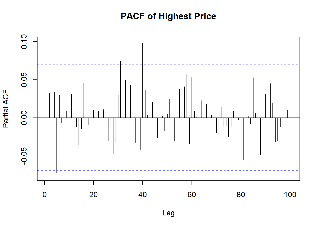
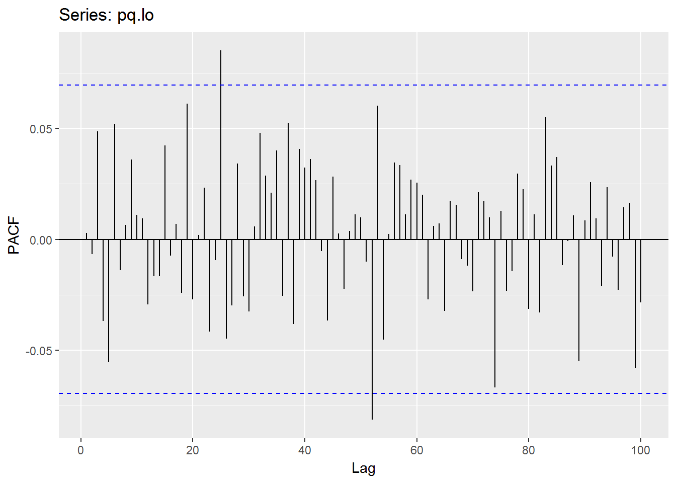
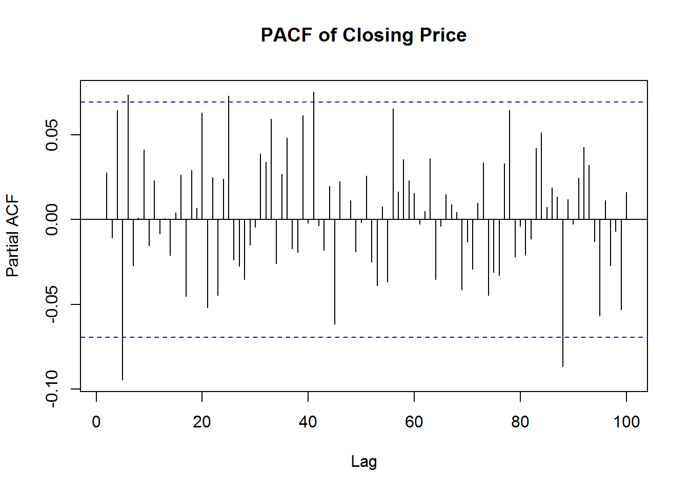
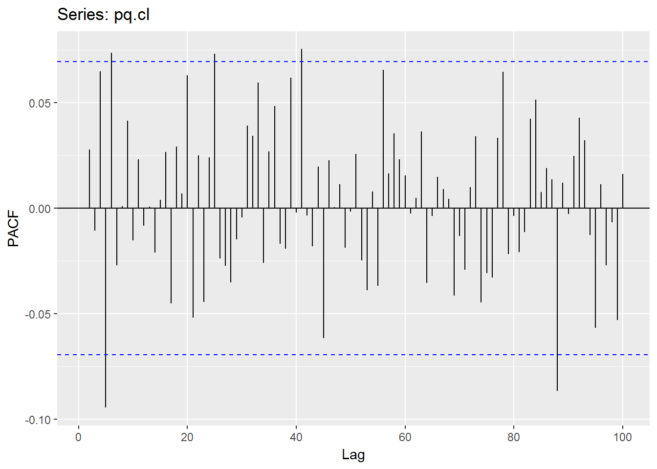
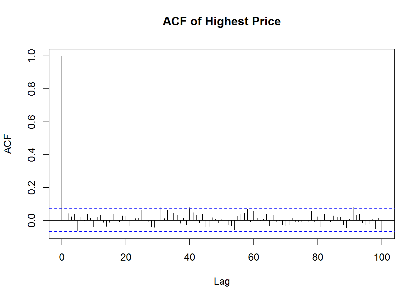
As I mentioned in first section which is the combination models will be more than 10,000, therefore I try to refer to acf() and pacf() to determine the best fit value p and q for ARMA model. You can refer to below articles for more information.
- 时间序列ARMA中p,q选择
- 时间序列分析之ARIMA模型预测__R篇13 Due to this article compare the combination models with
acfandpacfand eventually get thatacfandpacfproduce a better fit model. - Time Series Analysis of Apple Stock Prices Using GARCH models
- 时间序列建模问题,如何准确的建立时间序列模型?
- Arima预测模型(R语言)
- 时间序列分析—(ARIMA模型)
- Identifying the numbers of AR or MA terms in an ARIMA model
- 8.7 ARIMA modelling in R14 (a) The best model (with smallest AICc) is selected from the following four: 15 ARIMA(2,d,2), 16 ARIMA(0,d,0), 17 ARIMA(1,d,0), 18 ARIMA(0,d,1).
- 2.2 Partial Autocorrelation Function (PACF)
- Forecasting Time Series
- Lecture 4: Modelling Volatility of S&P returns
- Course Files :: MPO1 & MPO1A
- 第二章平稳时间序列模型——ACF和PACF和样本ACF/PACF
## Multiple Garch models inside `rugarch` package.
.variance.model.par <- c('sGARCH', 'fGARCH', 'eGARCH', 'gjrGARCH', 'apARCH', 'iGARCH', 'csGARCH', 'realGARCH')

## http://blog.csdn.net/desilting/article/details/39013825
## 接下来需要选择合适的ARIMA模型,即确定ARIMA(p,d,q)中合适的 p、q 值,我们通过R中的“acf()”和“pacf”函数来做判断。
#'@ .garchOrder.par <- expand.grid(0:2, 0:2, KEEP.OUT.ATTRS = FALSE) %>% mutate(PP = paste(Var1, Var2))
#'@ .garchOrder.par %<>% .$PP %>% str_split(' ') %>% llply(as.numeric)

.solver.par <- c('hybrid', 'solnp', 'nlminb', 'gosolnp', 'nloptr', 'lbfgs')

.sub.fGarch.par <- c('GARCH', 'TGARCH', 'AVGARCH', 'NGARCH', 'NAGARCH', 'APARCH', 'GJRGARCH', 'ALLGARCH')

.dist.model.par <- c('norm', 'snorm', 'std', 'sstd', 'ged', 'sged', 'nig', 'ghyp', 'jsu')

pp <- expand.grid(c('Op', 'Hi', 'Mn', 'Lo', 'Cl'), c('Op', 'Hi', 'Mn', 'Lo', 'Cl')) %>% mutate(PP = paste(Var1, Var2)) %>% .$PP %>% str_split(' ')
pp <- llply(pp, function(x) x[x[1]!=x[2]][!is.null(x)])
pp <- pp[!is.na(pp)]

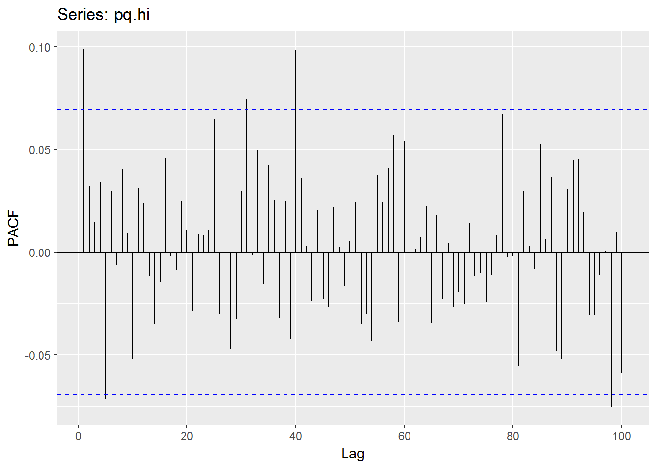
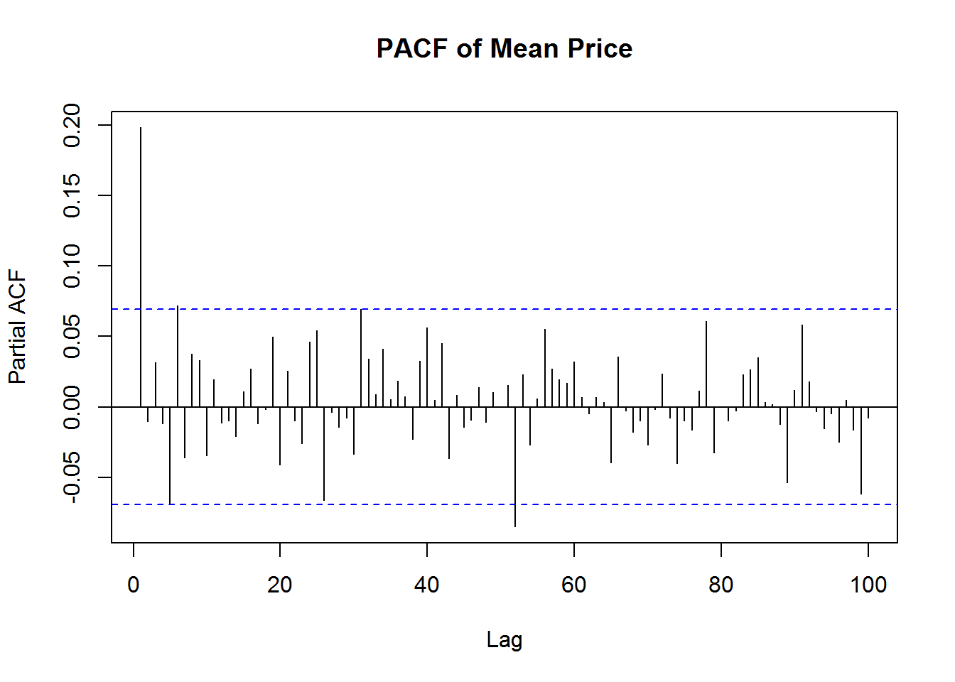
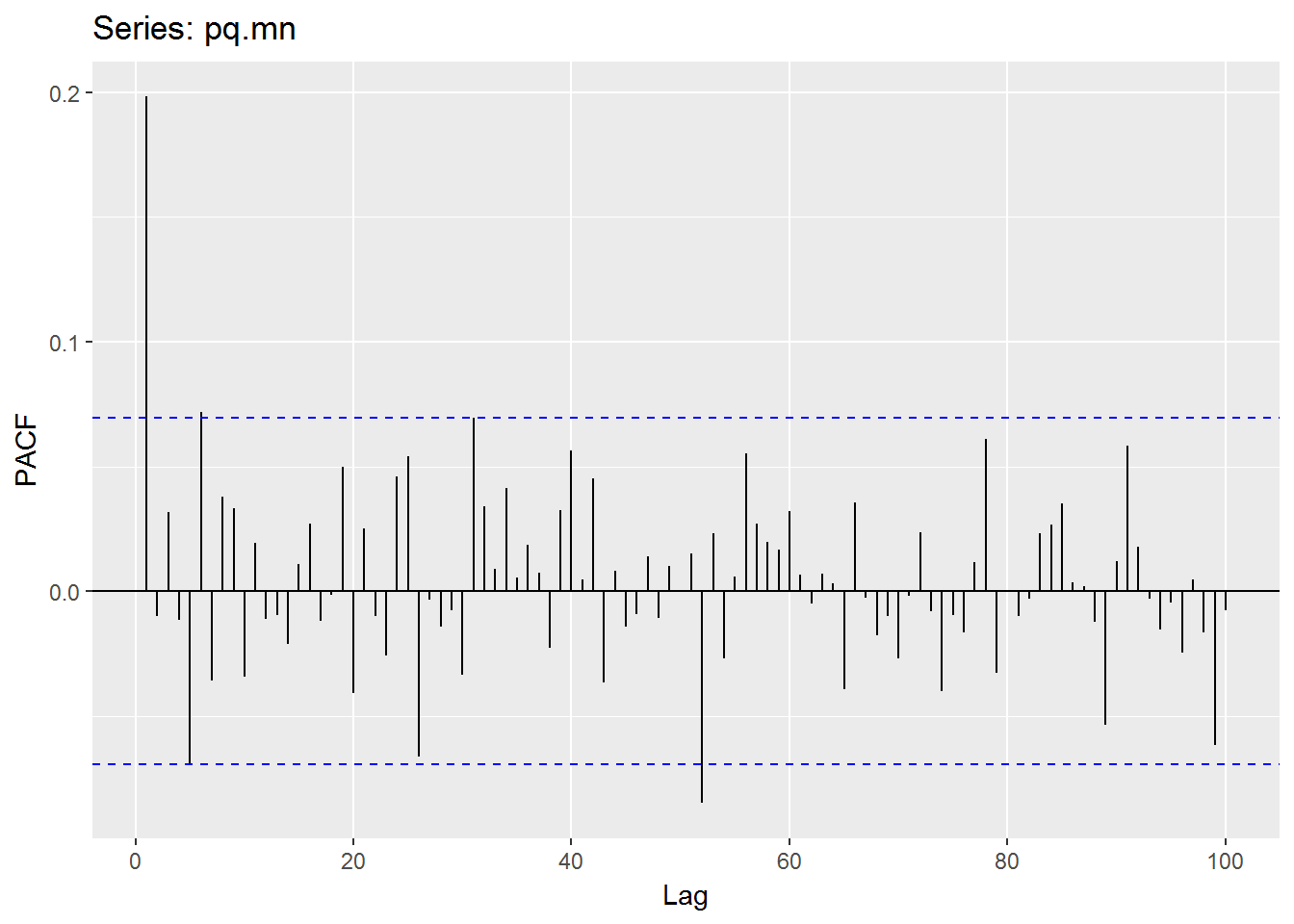
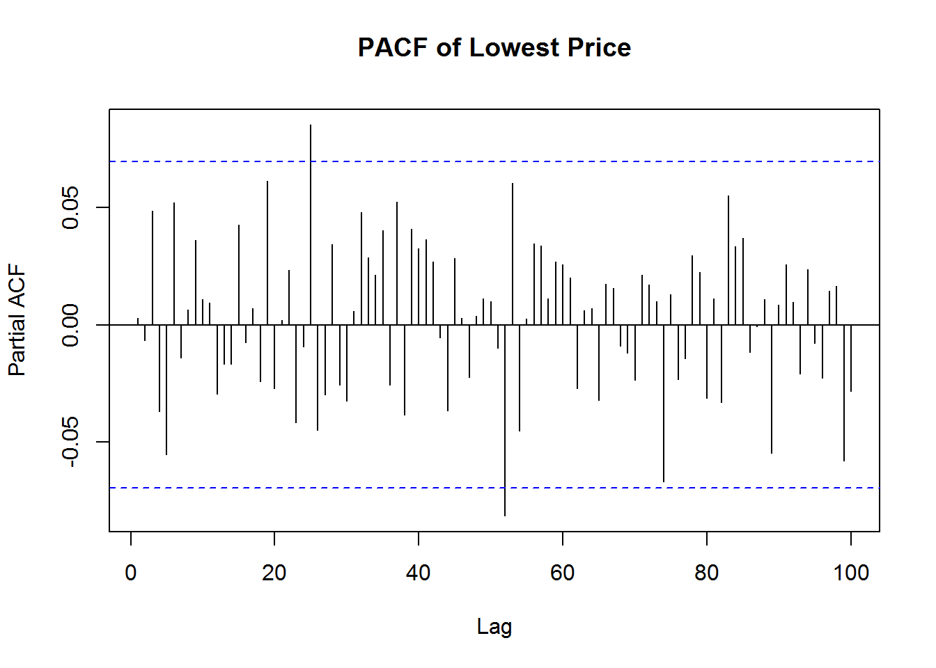


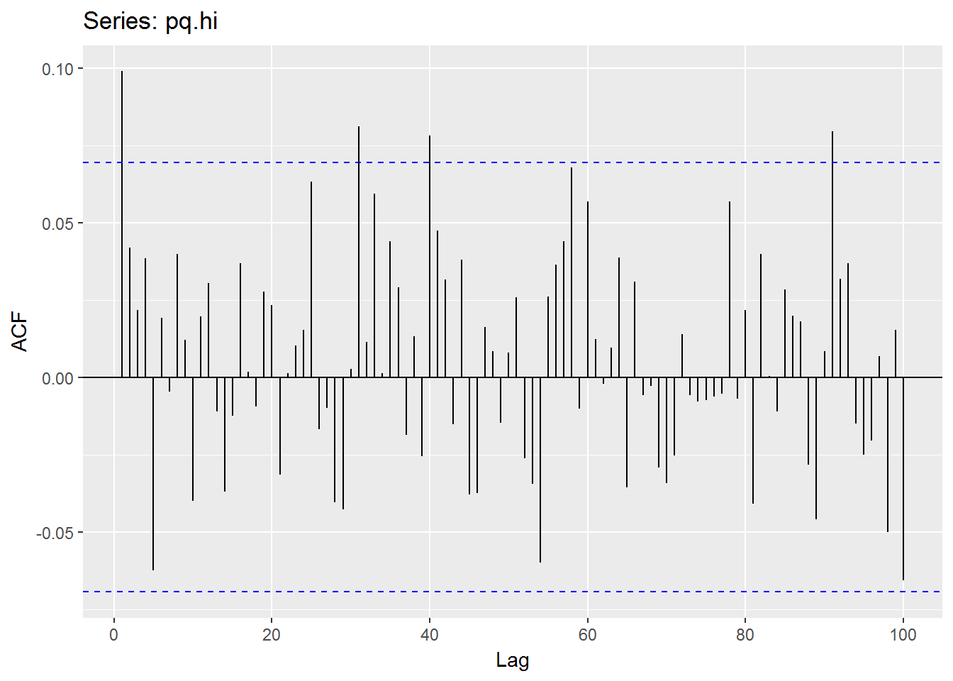

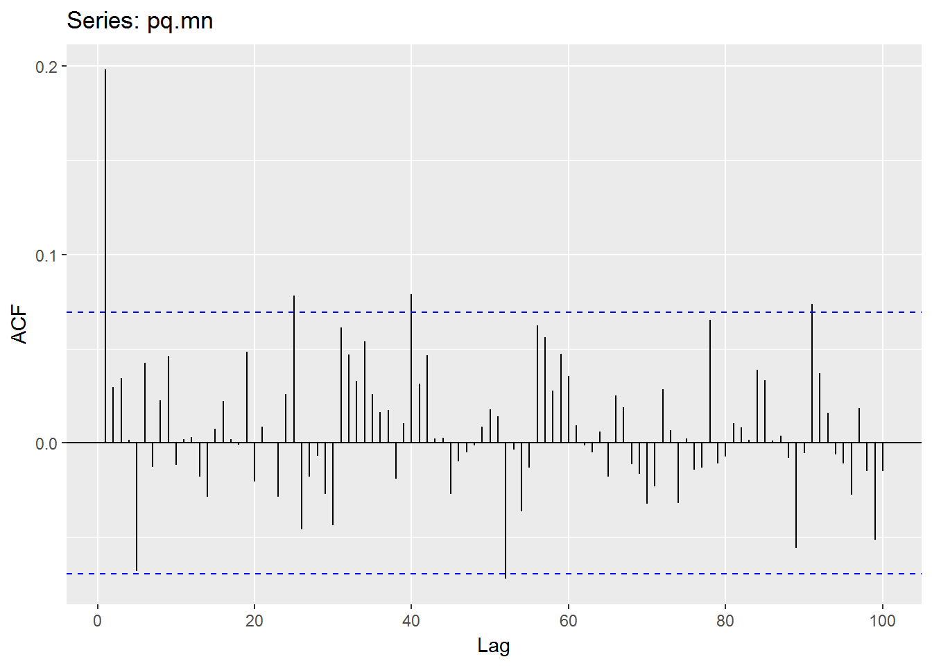
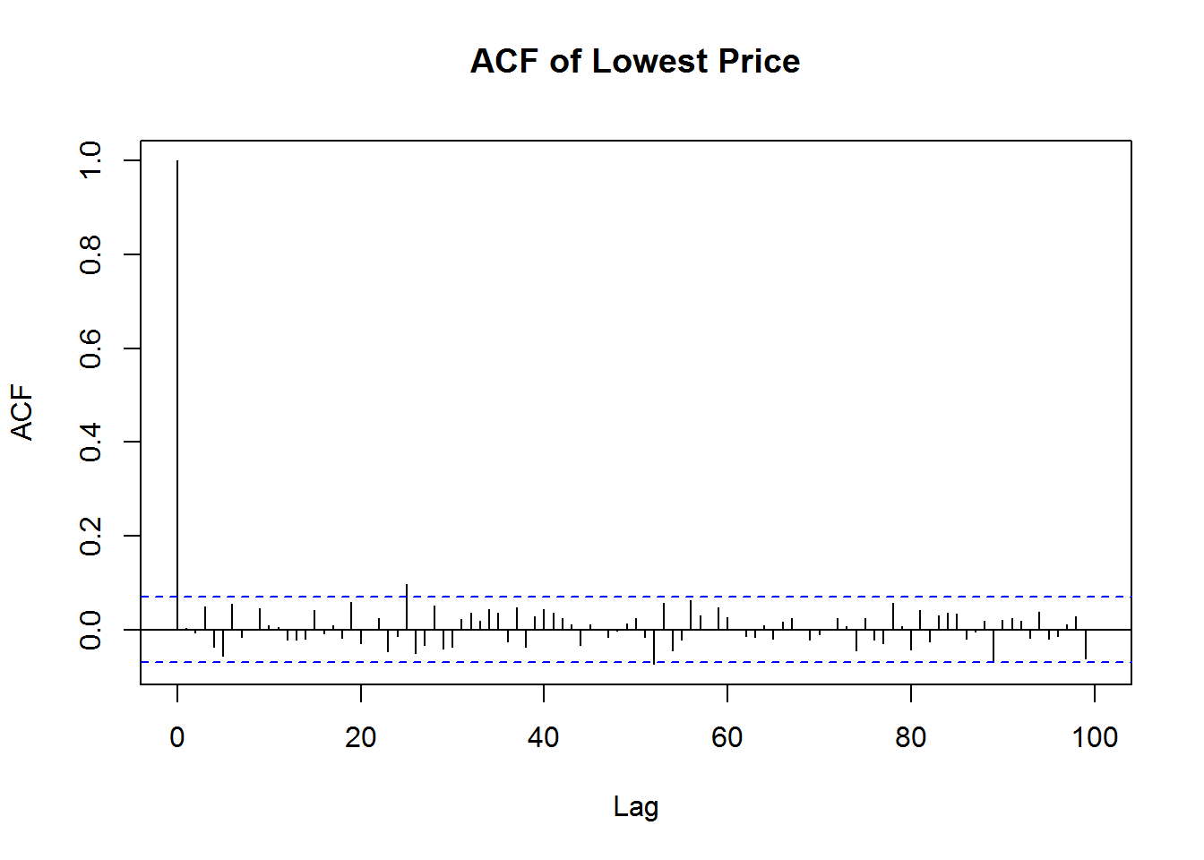
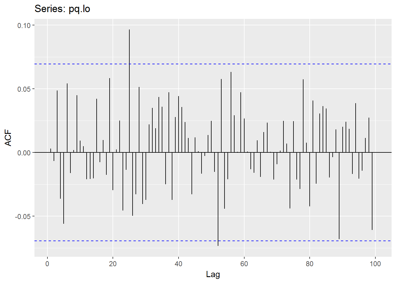
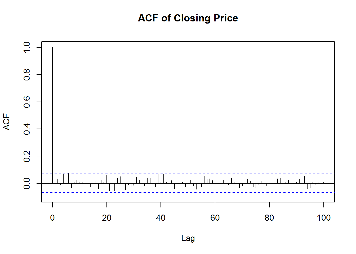
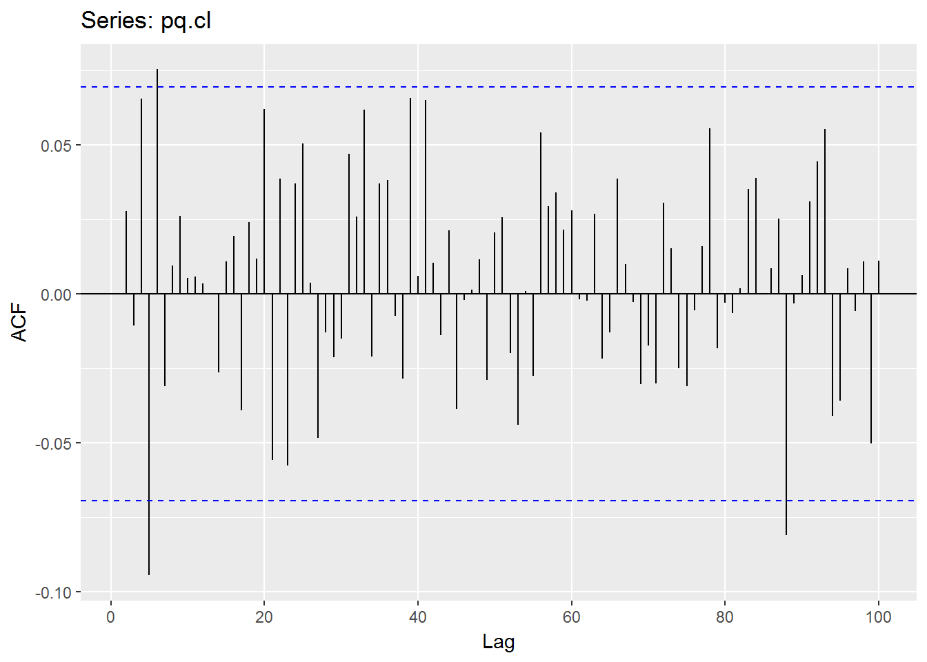
Here I use a function to find the optimal value of p and q from armaOrder(0,0) to armaOrder(5,5) by refer to R-ARMA(p,q)如何选找最小AIC的p,q值.
However, due to optimal r and s for Garch model will consume alot of time to test the optimal garchOrder(r,s) here I skip it and just using default garchOrder(1,1).
- An ARMA(p,q) model specifies the conditional mean of the process
- The GARCH(r,s) model specifies the conditional variance of the process
Kindly refer to What is the difference between GARCH and ARMA? for more information.
pq.op <- suppressWarnings(armaSearch(Op(mbase)))## method = 'CSS-ML', the min AIC = 1623.45338140965, p = 4, q = 4pq.hi <- suppressWarnings(armaSearch(Hi(mbase)))## method = 'CSS-ML', the min AIC = 1490.07263872323, p = 4, q = 3USDJPY.Mean = (Hi(mbase) + Lo(mbase)) / 2
names(USDJPY.Mean) <- 'USDJPY.Mean'
pq.mn <- suppressWarnings(armaSearch(USDJPY.Mean))## method = 'CSS-ML', the min AIC = 1369.50193310379, p = 3, q = 2pq.lo <- suppressWarnings(armaSearch(Lo(mbase)))## method = 'CSS-ML', the min AIC = 1710.3744852797, p = 2, q = 2pq.cl <- suppressWarnings(armaSearch(Cl(mbase)))## method = 'CSS-ML', the min AIC = 1634.7817779015, p = 3, q = 3## From below comparison, we know that the 'CSS-ML' is better than 'ML'.
##
#'@ > suppressWarnings(armaSearch(Cl(mbase)))
# the min AIC = 1635.718 , p = 2 , q = 4
# p q AIC
# 1 0 0 1641.616
# 2 0 1 1643.616
# 3 0 2 1645.062
# 4 0 3 1647.036
# 5 0 4 1645.792
# 6 0 5 1639.704
# 7 1 0 1643.616
# 8 1 1 1645.616
# 9 1 2 1640.169
# 10 1 3 1640.896
# 11 1 4 1636.914
# 12 1 5 1636.216
# 13 2 0 1644.991
# 14 2 1 1640.297
# 15 2 2 1642.826
# 16 2 3 1644.150
# 17 2 4 1635.718
# 18 2 5 1637.614
# 19 3 0 1646.901
# 20 3 1 1641.620
# 21 3 2 1643.541
# 22 3 3 1646.957
# 23 3 4 1636.964
# 24 3 5 1639.715
# 25 4 0 1645.485
# 26 4 1 1639.150
# 27 4 2 1635.929
# 28 4 3 1636.975
# 29 4 4 1638.584
# 30 4 5 1640.505
# 31 5 0 1640.214
# 32 5 1 1638.289
# 33 5 2 1637.855
# 34 5 3 1639.926
# 35 5 4 1638.875
# 36 5 5 1641.102
#'@ > suppressWarnings(armaSearch(Cl(mbase), .method = 'CSS-ML'))
# the min AIC = 1634.782 , p = 3 , q = 3
# p q AIC
# 1 0 0 1641.616
# 2 0 1 1643.616
# 3 0 2 1645.062
# 4 0 3 1647.036
# 5 0 4 1645.792
# 6 0 5 1639.704
# 7 1 0 1643.616
# 8 1 1 1645.616
# 9 1 2 1640.168
# 10 1 3 1640.896
# 11 1 4 1636.914
# 12 1 5 1636.216
# 13 2 0 1644.991
# 14 2 1 1640.297
# 15 2 2 1642.734
# 16 2 3 1643.207
# 17 2 4 1635.717
# 18 2 5 1636.222
# 19 3 0 1646.901
# 20 3 1 1641.620
# 21 3 2 1644.290
# 22 3 3 1634.782
# 23 3 4 1636.240
# 24 3 5 1638.113
# 25 4 0 1645.485
# 26 4 1 1639.150
# 27 4 2 1635.929
# 28 4 3 1636.975
# 29 4 4 1638.584
# 30 4 5 1640.505
# 31 5 0 1640.214
# 32 5 1 1638.289
# 33 5 2 1637.855
# 34 5 3 1639.926
# 35 5 4 1636.145
# 36 5 5 1641.102
#'@ > suppressWarnings(armaSearch(Mn(USDJPY.Mean)))
# the min AIC = 1369.503 , p = 3 , q = 2
# p q AIC
# 1 0 0 1408.854
# 2 0 1 1379.128
# 3 0 2 1380.864
# 4 0 3 1382.213
# 5 0 4 1383.223
# 6 0 5 1377.906
# 7 1 0 1378.869
# 8 1 1 1380.755
# 9 1 2 1382.479
# 10 1 3 1384.072
# 11 1 4 1379.514
# 12 1 5 1378.089
# 13 2 0 1380.792
# 14 2 1 1382.634
# 15 2 2 1384.310
# 16 2 3 1384.559
# 17 2 4 1375.647
# 18 2 5 1377.609
# 19 3 0 1381.965
# 20 3 1 1383.946
# 21 3 2 1369.503
# 22 3 3 1376.475
# 23 3 4 1377.613
# 24 3 5 1379.641
# 25 4 0 1383.859
# 26 4 1 1385.411
# 27 4 2 1375.856
# 28 4 3 1373.091
# 29 4 4 1378.873
# 30 4 5 1380.859
# 31 5 0 1382.015
# 32 5 1 1379.627
# 33 5 2 1377.687
# 34 5 3 1379.462
# 35 5 4 1380.859
# 36 5 5 1382.397
#
#'@ > suppressWarnings(armaSearch(Mn(USDJPY.Mean), .method = 'CSS-ML'))
# Show Traceback
#
# Rerun with Debug
# Error in arima(data, order = c(p, 1, q), method = .method) :
# non-stationary AR part from CSS
#
#'@ > suppressWarnings(armaSearch(Mn(USDJPY.Mean), .method = 'CSS'))
# the min AIC = , p = , q =
# p q AIC
# 1 0 0 NA
# 2 0 1 NA
# 3 0 2 NA
# 4 0 3 NA
# 5 0 4 NA
# 6 0 5 NA
# 7 1 0 NA
# 8 1 1 NA
# 9 1 2 NA
# 10 1 3 NA
# 11 1 4 NA
# 12 1 5 NA
# 13 2 0 NA
# 14 2 1 NA
# 15 2 2 NA
# 16 2 3 NA
# 17 2 4 NA
# 18 2 5 NA
# 19 3 0 NA
# 20 3 1 NA
# 21 3 2 NA
# 22 3 3 NA
# 23 3 4 NA
# 24 3 5 NA
# 25 4 0 NA
# 26 4 1 NA
# 27 4 2 NA
# 28 4 3 NA
# 29 4 4 NA
# 30 4 5 NA
# 31 5 0 NA
# 32 5 1 NA
# 33 5 2 NA
# 34 5 3 NA
# 35 5 4 NA
# 36 5 5 NA
#'@ > pq.op <- suppressWarnings(armaSearch(Op(mbase)))
# the min AIC = 1623.453 , p = 4 , q = 4
#'@ > pq.hi <- suppressWarnings(armaSearch(Hi(mbase)))
# the min AIC = 1490.073 , p = 4 , q = 3
#'@ > USDJPY.Mean = (Hi(mbase) + Lo(mbase)) / 2
#'@ > names(USDJPY.Mean) <- 'USDJPY.Mean'
#'@ > pq.mn <- suppressWarnings(armaSearch(USDJPY.Mean))
# the min AIC = 1369.503 , p = 3 , q = 2
#'@ > pq.lo <- suppressWarnings(armaSearch(Lo(mbase)))
# the min AIC = 1711.913 , p = 3 , q = 2
#'@ > pq.cl <- suppressWarnings(armaSearch(Cl(mbase)))
# the min AIC = 1634.782 , p = 3 , q = 3Paper Multivariate DCC-GARCH Model -With Various Error Distributions applied few error distribuions onto dcc-garch model (I leave the multivariate Garch for future works):-
- multivariate Gaussian
- Student’s t
- skew Student’s t
Below are the conclusion from the paper.
In this thesis we have studied the DCC-GARCH model with Gaussian, Student’s t and skew Student’s t-distributed errors. For a basic understanding of the GARCH model, the univariate GARCH and multivariate GARCH models in general were discussed before the DCC-GARCH model was considered…
After precenting the theory, DCC-GARCH models were fit to a portfolio consisting of European, American and Japanese stocks assuming three different error distributions; multivariate Gaussian, Student’s t and skew Student’s t. The European, American and Japanese series seemed to have a bit different marginal distributions. The DCC-GARCH model with skew Student’s t-distributed errors performed best. But even the DCC-GARCH with skew Student’s t-distributed errors did explain all of the asymmetry in the asset series. Hence even better models may be considered. Comparing the DCC-GARCH model with the CCC-GARCH model using the Kupiec test showed that the first model gave a better fit to the data.
There are several possible directions for future work. It might be better to use other marginal models such as the EGARCH, QGARCH and GJR GARCH, that capture the asymmetry in the conditional variances. If the univariate GARCH models are more correct, the DCC-GARCH model might yield better results. Other error distributions, such as a Normal Inverse Gaussian (NIG) might also give a better fit. When we fitted the Gaussian, Student’s t- and skew Student’s t-distibutions to the data, we assumed all the distributions to be the same for the three series. This might be a too restrictive criteria. A model where the marginal distributions is allowed to be different for each of the asset series might give a better fit. One then might use a Copula to link the marginals together.
dstGarch <- readRDS('./data/dstsGarch.Mn.Cl.rds')
dst.m <- ldply(dstGarch, function(x) x %>% dplyr::select(BR, Profit, Bal, RR) %>% tail(1)) %>% mutate(BR = 1000, Profit = Bal - BR, RR = Bal / BR)
#    .id   BR   Profit      Bal       RR
#1  norm 1000 182.7446 1182.745 1.182745
#2 snorm 1000 202.8955 1202.895 1.202895
#3   std 1000 155.7099 1155.710 1.155710
#4  sstd 1000 143.0274 1143.027 1.143027
#5   ged 1000 135.8819 1135.882 1.135882
#6  sged 1000 143.1829 1143.183 1.143183
#7   nig 1000 163.9009 1163.901 1.163901
#8  ghyp 1000 137.0740 1137.074 1.137074
#9   jsu 1000 178.7324 1178.732 1.178732

dst.m %>% kable(width = 'auto')| .id | BR | Profit | Bal | RR |
|---|---|---|---|---|
| norm | 1000 | 182.7446 | 1182.745 | 1.182745 |
| snorm | 1000 | 202.8955 | 1202.895 | 1.202895 |
| std | 1000 | 155.7099 | 1155.710 | 1.155710 |
| sstd | 1000 | 143.0274 | 1143.027 | 1.143027 |
| ged | 1000 | 135.8819 | 1135.882 | 1.135882 |
| sged | 1000 | 143.1829 | 1143.183 | 1.143183 |
| nig | 1000 | 163.9009 | 1163.901 | 1.163901 |
| ghyp | 1000 | 137.0740 | 1137.074 | 1.137074 |
| jsu | 1000 | 178.7324 | 1178.732 | 1.178732 |
From above comparison of distribution used, we know that snorm distribution generates most return (notes : I should use LoHi instead of MnCl since it will generates highest ROI, however most of LoHi Garch models facing large data size or large NA values error. Here I skip the LoHi data for comparison). Now we know the best p and q, solver using hybrid, and best fitted distribution. Now we try to compare the Garch models.
For dcc-Garch models which are multivariate Garch models will be future works :
- Multivariate GARCH(1,1) in R
- Multivariate volatility forecasting (1)
- Multivariate volatility forecasting, part 2 – equicorrelation
- The GARCH-DCC Model and 2-stage DCC(MVT) estimation
Below is the summary of ROI of Garch and EWMA by Kelly models.
Profit and Loss of Investment
Annual Stakes and Profit and Loss of Firm A at Agency A (2011-2015) ($0,000)
Volatility Staking
| Date | csGARCH.Bal | fGARCH.GARCH.Bal | fGARCH.NGARCH.Bal | gjrGARCH.Bal | gjrGARCH.EWMA.est.Bal | gjrGARCH.EWMA.fixed.Bal | iGARCH.Bal | iGARCH.EWMA.est.Bal | iGARCH.EWMA.fixed.Bal | realGARCH.Bal | |
|---|---|---|---|---|---|---|---|---|---|---|---|
| 530 | 2017-01-13 | -1000 | -200 | -200 | 800 | 800 | 800 | -1800 | -1800 | -1800 | -28800 |
| 531 | 2017-01-16 | -1100 | -300 | -300 | 700 | 700 | 700 | -1900 | -1900 | -1900 | -28900 |
| 532 | 2017-01-17 | -1000 | -200 | -200 | 800 | 800 | 800 | -1800 | -1800 | -2000 | -29000 |
| 533 | 2017-01-18 | -1100 | -300 | -300 | 700 | 700 | 700 | -1900 | -1900 | -2100 | -29100 |
| 534 | 2017-01-19 | -1000 | -200 | -200 | 800 | 800 | 800 | -1800 | -1800 | -2000 | -29200 |
| 535 | 2017-01-20 | -1100 | -300 | -300 | 700 | 700 | 700 | -1900 | -1900 | -2100 | -29300 |